Linear Algebra is the study of Vector Spaces

Vectors and Vector Spaces

Vector Space
An Algebraic Structure containing Tensor elements called Vectors, over a Algebraic Field of Scalar values.

Vector Space Element
Note that Vectors need not be . Any possible element of a vector space is by definition, a vector. This means that vector spaces really contain Tensors. 99% of the time when people are talking about vectors, they really mean “Coordinate vector”, i.e. a vector that represents a location in Space. Whereas a vector represents a location in a Vector Space.
Link to original

Axioms

The Axioms neccessary to qualify as a Vector Space are

Abelian Group under Addition

Scalar Multiplication

Abelian Group under Addition Axioms

Closure:

Associativity:

Identity:

Inverse:

Commutativity: Scalar Multiplication Axioms

Closure:

Associativity:

Distributivity:

Distributivity:

Link to original

Vector
An element of a Vector Space, represented in that space either by a direction and magnitude, or by a list of Numbers, each describing the placement along a coordinate axis.

Circular transclusion detected: Mathematics/Algebra/LinearAlgebra/Vector-Space-Element

Operations

Addition

Add elementwise.

Subtraction

Subtract elementwise.

Scalar Multiplication

Multiply elementwise.

Magnitude

The magntiude calculates the distance from the tip of the vector to the origin.

Dot Product

Transclude of Dot-Product

Cross Product

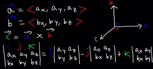
Transclude of Cross-Product
Link to original

Subspaces of

Subspace
A Vector Space’s version of a Subset, with some constraints.

While, a subspace does inherit the axioms of a Vector Space. Verifying a subset is a subspace is simpler; A Subset of is a subspace if it is closed within scalar multiplication and vector addition:

Properties

, i.e. the Span of any subset is identical to itself

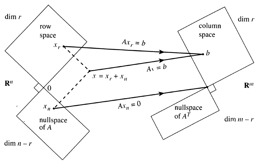
Four Fundamental Subspaces

For Matrix

The Subspaces are linked by the Fundamental Theorem of Linear Algebra

Rowspace

Nullspace of

Columnspace

Nullspace of , “Left Nullspace”

Shows the relationship between the dimensions of the subspaces

Shows the Morphisms between different subspaces of a matrix

Show existence of solutions:

Shows the Orthogonality relationship between related subspaces of a matrix

Link to original

Columnspace
The Subspace defined by the Span of the columns of Matrix

See Rank
Link to original

Rowspace
The Subspace defined by the Span of the rows of Matrix
Link to original

Nullspace
The Subspace defined by the Set of that satisfy

See Nullity
Link to original

Basis
A Set of Basis Vectors. A set of Linearly Indepedent Vectors whose Linear Combinations can represent any vector in that space.

Standard Basis Vectors in are i, j, k, but you can use other vectors to span the same amount of space if you want.

Let

is some basis for the subspace

Dimension
The dimension of a Subspace is the Cardinality of its Basis

This is because a basis requires a Set of Linearly Indepedent Vectors, and does not meet this requirement. Therefore, its only basis is . The cardinality of the empty set is 0, therefore so is

Examples

dim

dim(Nul A) is the number of

number of free vars of A

dim(Col A) is the number of

number of pivots of A

H =

n variables, solve for ito everything else. → one pivot everything else free vars. Therefore free vars

Link to original

Basis Theorem
Any two bases for a Subspace have the same Dimension
Link to original
Link to original

Rank

the rank of a matrix A is the dimension of its Columnspace

number of Pivots

Link to original

Nullity

The nullity of a matrix is the dimension of its Nullspace

The number of Free Variables

Link to original

Fundamental Theorem of Linear Algebra
Link to original

Invertibility Theorem
A is an , Square Matrix A is Invertible The columns of A are a Basis for Col A = rank A = dim Col A = n nullity A = dim Nul A = 0 Nul A = {}
Link to original

Determinant
Imagine the area of parallelogram created by the basis of a standard vector space, like . Now apply a linear transformation to that vector space. The new area of the new parallelogram has been scaled by a factor of the determinant. is the parallelopiped.

You can also just think of it as the area of the parallelogram spanned by the columns of a matrix

: parallelopiped and volume

(assume n by n matrix because we only know how to find determinants for square matrices)

You can also get the area of S by using the determinant of the matrix created by the vectors that span S, i.e. because you are shifting the standard basis vectors into the vector space dictated by S

Determinant Laws

det(A) = 0 A is singular

det(A) 0 A is invertible

det(Triangular) = product of diagonals

det A = det

det(AB) = det A · det B

Determinant Post Row Operations

if A square:

if adding rows to rows on A to get B then

if swapping rows in A to get B then

if scaling one row of A by k, then = Exactly the same for columns

Link to original

Cofactor Expansion
Cofactor expansion is a method used to calculate the Determinant of an matrix . It works by reducing the determinant of the matrix to a sum of determinants of submatrices. It is a recursive definition.

where is the determinant of the submatrix of obtained by deleting the -th row and -th column

The signs for each term of the expansion are determined solely by the position and follow a checkerboard pattern, starting with in the top-left corner

The determinant of a matrix can be calculated by cofactor expansion along any single row or any single column .

Expansion Along Row :

Expansion Along Column :

Strategy: To simplify calculations, it is generally best to choose the row or column with the most zeros.
Link to original

Eigenstuff
Eigenvectors and Eigenvalues

Given

A is square

defined, e.g. if then

Eigenvector

is an eigenvector for An eigenvector is a vector solution to the above equation, such that the linear transformation of has the same result as scaling the vector by .

Eigenvalue

is the corresponding eigenvalue () Solve for in , which yields the Characteristic Equation for this system, e.g. in a 2D systems it is . In a 3D+ system, you still have to create the characteristic equation but it requires

Notes:

point same direction

point opposite direction

can be complex even if nothing else in the equation is

Eigenvalues cannot be determined from the reduced version of a matrix ⭐

i.e. row reductions change the eigenvalues of a matrix

The diagonal elements of a triangular matrix are its eigenvalues.

A invertible iff 0 is not an eigenvalue of A.

Stochastic matrices have an eigenvalue equal to 1.

If are eigenvectors that correspond to distinct eigenvalues, then are linearly independent

Defective

An eigenvalue is defective if and only if it does not have a complete Set of Linearly Independent eigenvectors.
Due to ‘s contribution,

Neutral Eigenvalue

Eigenspace

the span of the eigenvectors that correspond to a particular eigenvalue

Link to original

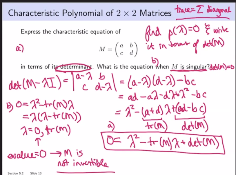
Characteristic Equation
to get values for . Recall means noninvertible. If a matrix isn’t invertible, then we won’t get trivial solutions when solving. Also the idea of reducing the dimension through the transformation is relevant; squishing the basis vectors all onto the same span where the area/volume is 0. Recall eigenvectors remain on the same span despite a linear transformation.

is an eigenvalue of A is singular

trace of a Matrix is the sum of diagonal

Characteristic Polynomial

n degree polynomial → n roots → maximum n eigenvalues (could be repeated)

Algebraic Multiplicity

Algebraic multiplicity of an eigenvalue is how many times an eigenvalue repeatedly occurs as the root of the characteristic polynomial.

Geometric Multiplicity

Geometric multiplicity of an eigenvalue is the number of eigenvectors associated with an eigenvalue; , which is saying how many eigenvector solutions does this eigenvalue have (recall is number of free vars in )

Link to original

Similar

square matrices A,B are similar we can find P so that

A,B similar same Characteristic Polynomial same eigenvalues

Link to original

Systems of Linear Equations

Linear System
A system of Linear Equations.

Representation

There are several equivalent ways to represent a linear system.

A system of Equations

An Augmented Matrix

A Vector Equation

A Matrix Equation
Link to original

Linear Equation

An Equation where in the above form where the the a’s are coefficients, x’s are variables, n is the dimension (number of variables), e.g. has two dimensions
Link to original

Row Reduction
Row Operation

Row Operation

Replacement/Addition

Interchange

Scaling Row operations can be used to solve systems of linear equations

Single row operations can be represented by an Elementary Matrix A system of equations written as an Augmented Matrix

Row operation example (these are augmented)
Link to original

Consistent

A linear system is considered consistent if it has solution(s)

Theorem for Consistency

A linear system is consistent iff the last column of the augmented matrix does not have a pivot. This is the same as saying that the RREF of the augmented matrix does not have a row of the form

Moreover, if a linear system is consistent, then it has 1. a unique solution iff there are no free variables. 2. infinitely many solutions that are parameterized by free variables

Row Equivalent

Row Equivalent
If two matrices are row equivalent they have the same solution set, meaning that they have a Bijection through Row Operations
Link to original

Echelon Form

Echelon Form
A rectangular matrix is in echelon form if

If there are any, all zero rows are at the bottom

The first non-zero entry (leading entry) of a row is to the right of any leading entries in the row above it

All elements below a leading entry are zero For reduced row echelon form

All leading entries, if any, are equal to 1.

Leading entries are the only nonzero entry in their respective column.

Pivot

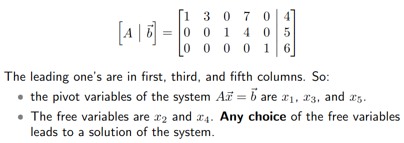
A Pivot in a matrix A is a location in A that corresponds to a leading 1 in the RREF of A

A Pivot column is the column of the pivot

Free Variable

Free variables are the variables of the non-pivot columns

Any choice of the free variables leads to a solution of the system

If you have any free variables you do not have a unique solution]

Link to original
Link to original

Vector Equations

Vector Equation
An Equation comprised of Vectors, rather than Scalars.

For example, the vector equation of a Space Curve through
Link to original

Real Number
A Real Number is a Number that represents a continuous quantity.

is all real numbers

Contains , the Set of Rational Numbers

is dimensions of

is rows and columns

Link to original

Linear Combination
Let is a linear combination of the vectors, with weights of the ‘s
Link to original

Span

The Set of all Linear Combinations of the ‘s in called the span of the ‘s

e.g.

any 2 vectors in that are not scalar multiplies of each other span Q: Is

Link to original

Homogenous
When an Equation has a “trivial” solution or

Homogenous System

Homogenous System
Homogenous systems always have a trivial solution, so naturally we would like to know if there are nontrivial, perhaps infinite solutions, namely if there is a free variable and a column with no pivots
Link to original

Homogenous Differential Equation

Homogeneous Differential Equation
A Linear Differential Equation satisfied by .
Link to original
Link to original

Linear Independence
Linear Independence

The only solution to is the trivial Linearly Independent

Geometric Interpretation

If two vectors are linearly independent, the are not colinear If 3, then not coplanal If 4, not cospacial

Linear Dependence

Any of the vectors in the set are a linear combination of the others

If there is a free variable, so there are infinite solutions to the homogenous equation

If the columns of A are in , and there are basis vectors in (which is always true), then if the amount of columns in A exceeds the amount of basis vectors that exist in that dimension, it means that there are free variables, which indicates linear dependence

If one or more of the columns of A is

Iff

Link to original

Intro to Linear Transformations

Linear Transformation
A Linear transformation is a Transformation where

where

Domain of T is (where we start)

Codomain or target of T is

The vector is the image of under T

The set of all possible images is called the range

image range codomain

When the domain and codomain are both , you can represent them as a Cartesian Graph in , as in a mapping of

If y is the codomain and x is the domain, the range is the range, the domain is all the images of f(x)

Addition Rule

T(u + v) = T(u) + T(v)

Multiplication Rule

T(c) = cT(v)

Prove a transformation is linear by proving the addition and multiplication rules.

“Principle of Superposition”

If we know , …, then we know every T(v)

1-1

Injective
If there is at most one location in the Codomain for every location in the Domain
Link to original

1-1 every column of T is a pivot column

1-1 iff standard matrix has pivot in every column

Onto

Surjective
If there is a location in the Codomain for every location in the Domain
Link to original

TLDR: Onto every row of T is a pivot row

onto iff the standard matrix has a pivot in every row

The matrix A has columns which span .

The matrix A has all pivotal rows.

Bijective

Bijective
If there is exactly one location in the Codomain for every location in the Domain for the Transformation
Link to original

Needs square matrix

Matrix Multiplication is a Linear Transformation

Compute

Calculate so that

Give a Give a that is not in the range of Give a that is not in the span of the columns of (Same question for all)

Range of is a bunch of images of the following form:

For to not be in the range of , it cannot be in the above form, e.g. it can be
Link to original

Matrix of Linear Transformations

The standard (basis) vectors

Circular transclusion detected: Mathematics/Algebra/LinearAlgebra/Basis

Basis Vector
A Vector that an element of a Basis for a Vector Space, which is a Set of Linearly Indepedent whose Linear Combinations can represent any vector in that space.

Standard Basis Vector

Standard basis vectors in that have a one entry for each dimension, and zeros for the rest,

e.g. for :

You could choose any basis for so long as it is linearly independent, but the standard basis for a dimension is the most convienient one

Link to original

Standard Matrix
A standard matrix is a Matrix that represents a Linear Transformation, where the transformation can be expressed as . It is found by applying the transformation to the Standard Basis Vectorss and using the results as the columns of the matrix

Theorem

Let be a Linear Transformation. Then there is a unique Matrix such that In fact, is a and its column is a vector

Example

Find standard matrix A for T(x) = 3 for x in
Link to original

Zero Matrix
A Matrix full of zeroes.

Multiplying any matrix by the zero matrix yields a zero matrix, though not neccessarily the same zero matrix

The Zero Vector is a special case

Link to original

Identity Matrix
A Matrix full of zeroes, except for ones on the diagonal.

Called the Identity matrix, because it follows the Multiplicative Identity Property

It is denoted as or to indicate , but is usually obvious based on context

Link to original

Circular transclusion detected: Mathematics/Algebra/LinearAlgebra/Zero-Matrix

Circular transclusion detected: Mathematics/Algebra/LinearAlgebra/Identity-Matrix

Matrix
A matrix is a rectangular array of Numbers

Operations

Matrix Addition

Add elementwise

Operand matrices must have the same dimensions

Matrix Multiplication

Let

Then, the entry of is , where we are performing many Dot Products to calculate the matrix product

Then

Multiplication Properties

Transpose

Transpose Properties

Inverse

Row reduce until you get for A

Keep track of the Elementary Matrix for each Row Operation

The product of all of the elementary matrices is the inverse of , by definition

may not be invertible. In this case, you won’t be able to row reduce it to the Identity Matrix

Invertible

You cannot always take the inverse of a matrix. Whether or not it is possible is called Invertibility. See also Invertible Matrix Theorem, Invertibility Theorem.

Invertibility Definition: is invertible if

A is invertible A is square

A is invertible it is row equivalent to the identity

Linearly dependent Singular

Mnemonic: After the trial, Johnny Depp was Single

Linearly independent Invertible

This is just the inverse of the above

is invertible

Basically means that A is Bijective

invertible

Inverse Properties

Inverse Shortcut
Link to original

Elementary Matrix
An elementary matrix, , is one that differs by by one Row Operation.
Link to original

Singular Matrix
A Matrix that is not Invertible
Link to original

Block Matrix
A Matrix that you write as a matrix of matrices

When doing multiplication with a block matrix, make sure the “receiving” matrix’s entries go first, to respect the lack of commutativity in matrix multiplication. See Multiplication
Link to original

LU Decomposition
If A is an Matrix that can be row reduced to Echelon Form without row exchanges, then

where is a composition of elementary matrices such that it is a Lower Triangular Matrix where all of its diagonal entries are 1

is an Echelon Form of

The Process

Suppose A can be row reduced to echelon form U without interchanging rows, i.e.

You can construct by finding each and multiplying them all together. Alternatively you can construct such that the sequence of row operations that convert to would convert to
Link to original

Markov chains

Probability Vector
Some Vector with nonnegative elements that sum to 1
Link to original

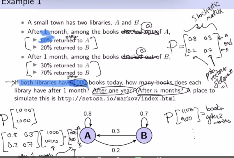
Stochastic Matrix
A stochastic matrix is a Square Matrix whose columns are Probability Vectors.

|det(P)| ⇐ 1, only volume contracting or preserving

Theorem as

If is a regular stochastic matrix, then has a unique steady-state vector , and converges to as ; where

Regular

Stochastic matrix is regular if there strictly has positive entries

Regular unique steady state vectors

Irregular steady state vectors

Link to original

Markov Chain
A Markov chain is a sequence of Probability Vectors, and a Stochastic Matrix P , such that:
Link to original

Diagonalization

Diagonalization
Diagonal Matrix

A matrix is diagonal if the only non-zero elements, if any, are on the main diagonal.

If is diagonal, then is very easy to compute because you simply exponentiate every diagonal element by

Diagonal matrices cannot have

Strang

Consider a matrix with some eigenvalues and eigenvectors. …

Diagonalizable

Orthogonal Diagonalization
Link to original

Diagonalizable
is diagonalizable, where is a diagonal matrix

is diagonalizable has linearly independent eigenvectors. i.e.

where vectors are linearly independent eigenvectors, and are the corresponding eigenvalues, in order.

Distinct Eigenvalues

If and has distinct eigenvalues, then is diagonalizable

Non-distinct Eigenvalues

You check that the sum of the geometric multiplicities is equal to the size of the matrix. e.g. for

Find the eigenvalues:

We know that geomult ⇐ algmult. Therefore has 1 distinct eigenvector. This means has to have 2 distinct eigenvectors to form a basis, so if it doesn’t then the matrix is not diagonalizable.

There is only one free columns here. Therefore, the dimension of the Nullspace is one, not two, which means the matrix is not diagonalizable.

Basis of Eigenvectors

Misc.
Link to original

Complex Eigenvalues

Complex Number
The Complex Numbers are a Number Set denoted by that extends the Real Numbers via the Imaginary Unit

is a Vector Space Isomorphism of

Like , the complex numbers can be represented within the Cartesian Plane.

is a closed Algebraic Field

Complex numbers are of the form

where

where is the Imaginary Unit

Euler's Formula

Consequence of Euler’s Identity

Suppose has an angle and has

The product has angle , and modulus

Link to original

Operations

Binary

Addition

Like adding Vectors in

Subtraction

Like subtracting Vectors in

Multiplication

Division

Unary

Real Component Function

Imaginary Component Function

Argument

Complex Conjugate

Reflects across the Real axis.

Magnitude

Also called “Modulus”

The magnitude is the in the figure.
Link to original

Circular transclusion detected: Mathematics/SetTheory/Complex-Number

Complex Eigenvalues

Complex Eigenstuff

Complex roots coming in complex conjugate pairs implies that complex Eigenvalues and their Eigenvectors come in complex conjugate pairs. This is because eigenvalues are the solutions to the Characteristic Equation, which is a Polynomial equation.
Link to original

Example

4 of the eigenvalues of a 7 x 7 matrix are -2, 4 + i, -4 - i, and i

Because there are 3 nonconjugate complex pairs, we know that the remaining eigenvalues are the conjugates of the given complex values
What is the characteristic polynomial?

Example

The matrix that rotates vectors by radians about the origin and then scales vectors by is:

What are the eigenvalues of ? Find an eigenvector for each eigenvalue

Could reason the eigenvalue for by the fact that eigenvalues and their eigenvectors come in complex conjugate pairs.

Orthogonal Sets

Orthogonal
Perpendicular.

and are orthogonal if

If is a subspace of and , is orthogonal to if it is orthogonal to every vector in

The set of all vectors orthogonal to a subspace is a itself a subspace, called the Orthogonal Complement of , , W perp

is orthogonal to each row of

is orthogonal complement to

number of columns

Link to original

Orthogonal Set
A Set of Vectors are an orthogonal set of vectors if every pair in the set is Orthogonal to every other vector in the set.

Linear Independence for Orthogonal Sets

If there is an orthogonal set of vectors , then

is Linearly Indepedent

Expansion in Orthogonal Basis

If is the Basis for Subspace in and is an orthogonal basis, then for any vector
Link to original

Orthogonal Projection
Link to original

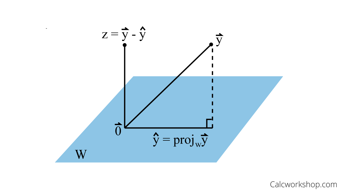
Orthogonal Decomposition
I proceed to define the orthogonal decomposition for some vector , where , where is a subspace of , where is the Orthogonal Complement of , where is the orthogonal projection of onto , and is a vector orthogonal to . This is a Vector Decomposition.

Every has a unique sum in the form above, so long as is a subspace of

Concerning

If is an Orthogonal Basis for , then , the orthogonal projection of onto is given by:

See Best Approximation, but in essence is the closest vector in to

Examples:

HW 6.3 Q1 HW 6.3 Q5 HW 6.3 Q6
Link to original

Best Approximation
is a subspace of , ,

In other words, is closest vector in to See Orthogonal Decomposition, especially for the visual interpretation of this.
Link to original

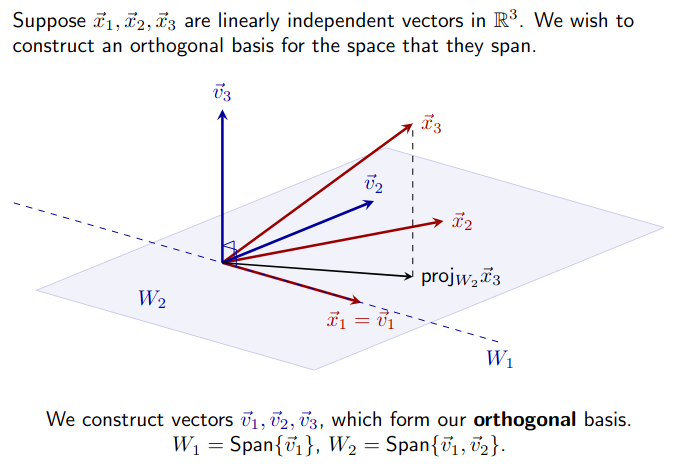
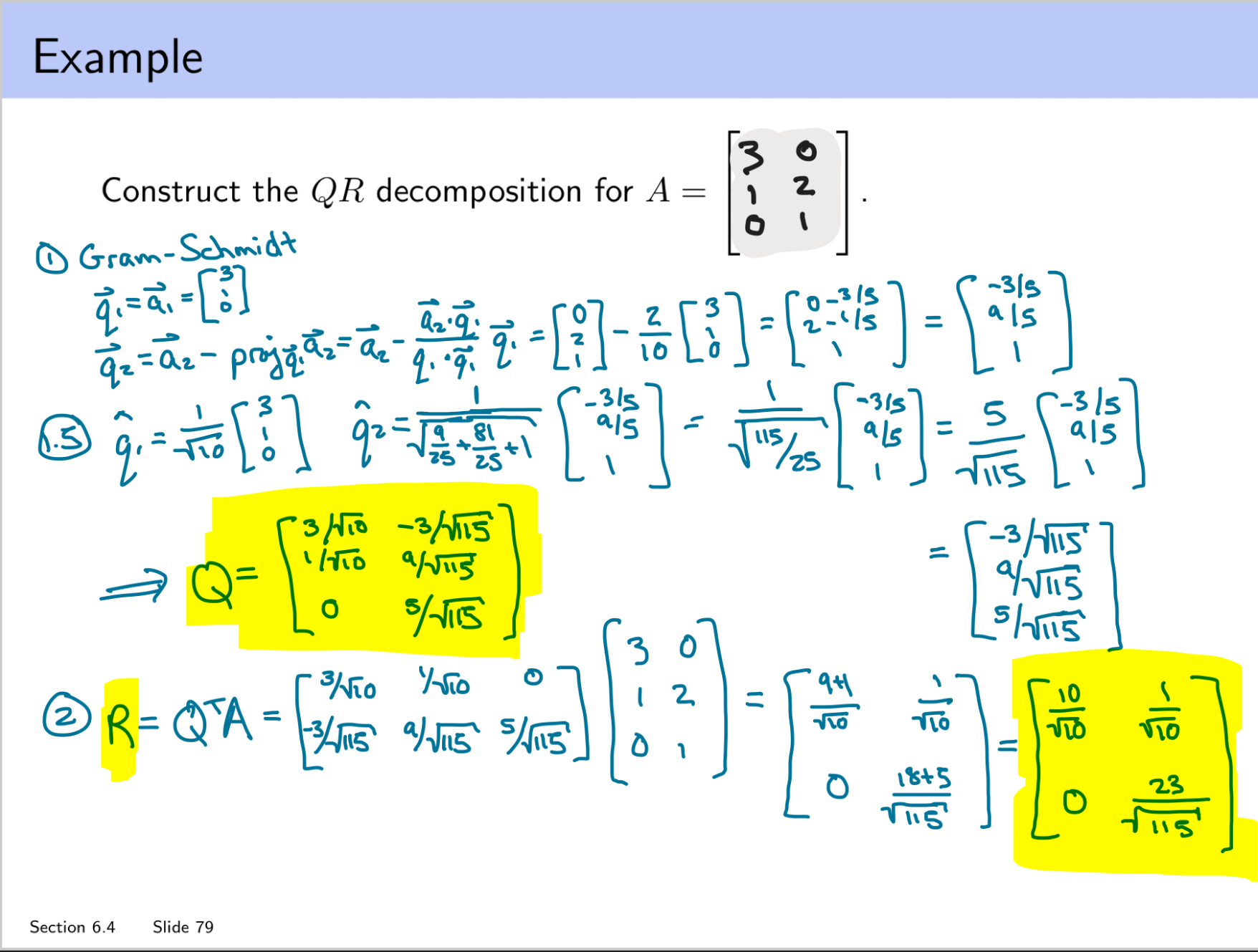
Gram-Schmidt Process
Let be a set of vectors that form a basis for subspace of , Let be a set of vectors that form an Orthogonal Basis for The Gram-Schmidt process defines how can be derived from It depends on Orthogonal Decomposition

If , iteratively define vectors in

Examples

HW 6.4 Q1 HW 6.4 Q2
Link to original

QR Decomposition
For any matrix , with Linearly Indepedent columns:

Q is

m x n

its columns are an orthonormal basis for Col A R is

n x n

upper triangular

positive diagonal

where and are columns of R and A

Link to original

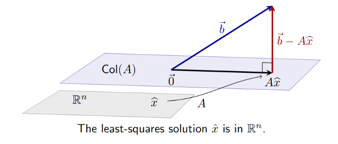
Least Squares
Given

Given many data points, construct a matrix equation in the form of a linear equation (this matrix equation will be overdetermined). The matrix equation below is This equation is linear but it doesn’t have to be, just adjust accordingly to represent the equations as a matrix equation.

Goal

Using Best Approximation, find a vector in subspace closest to

is a subspace of , , i.e. Note: Can only use Orthogonal Decomposition for when the columns of A form an orthogonal basis, by definition

In other words, is closest vector in to Note: is a unique vector, a special that minimizes the above equation. Note: If the columns of are orthogonal, then you can just use the scalar projection of onto each column of .

Normal Equations

The least squares solutions to corresponds to the solution to

Turns the equation from above and transforms it into a square matrix equation

Derivation

is the Least Squares Solution to

Normal Equation Usage

Use when non-square matrix

Over/Under determined

Regression

Theorem (Unique Solutions for Least Squares)

If A is m x n

Ax = b has a unique least squares solution for each b in Rm

Cols of A are linearly independent

The matrix A^T A is invertible If the above hold, the unique least square solution is

If the above conditions are not true, there may be infinitely many solutions, or some other nonunique amount of solutions, in which case you should consider instead.

Note: plays the role of the “length squared” of the matrix A

Theorem (Least Squares and QR)

Examples

Hampton Explanation for Least Squares

Let . is the unique, minimizing solution to the equation such that

Essentially, minimize

is the minimal distance between the different solutions

Goal: Find s.t. is closest to

in this context just denotes the special/unique that minimizes the distances between and b is closer to Axhat than to Ax for all other x in Col A

If b in Col A, then xhat is…

Seek so that is as close to as possible, i.e. should solve Axhat = bhat

Link to original

Google Page Rank
Stochastic Matrix
Link to original

Symmetric Matrix
Definition

Matrix A is symmetric if A^T = A

The eigenspaces of a symmetric matrix are orthogonal
Link to original

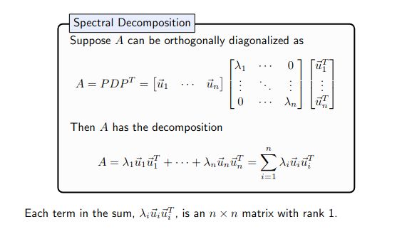
Spectral Decomposition
https://www.youtube.com/watch?v=mhy-ZKSARxI

Symmetric

Recall: If P is an orthogonal n × n matrix, then P −1 = P T , which implies A = PDP^T is diagonalizable and symmetric.

Spectral Thm

An n × n symmetric matrix A has the following properties.

All eigenvalues of A are real.

The dimenison of each eigenspace is full, that it’s dimension is equal to it’s algebraic multiplicity.

The eigenspaces are mutually orthogonal.

A can be diagonalized: A = PDP^T , where D is diagonal and P is orthogonal.

Spectal Decomp

Link to original

Orthogonal Diagonalization
Like Diagonalization, but you perform it on an orthogonal matrix, which makes the process easier as follows:

Where , i.e. is orthogonal It is otherwise the same as performing diagonalization on an arbitrary matrix
Link to original

Quadratic Form

Change of variable

Positive Definite Positive Semidefinite Negative Definite Negative Semidefinite
Link to original

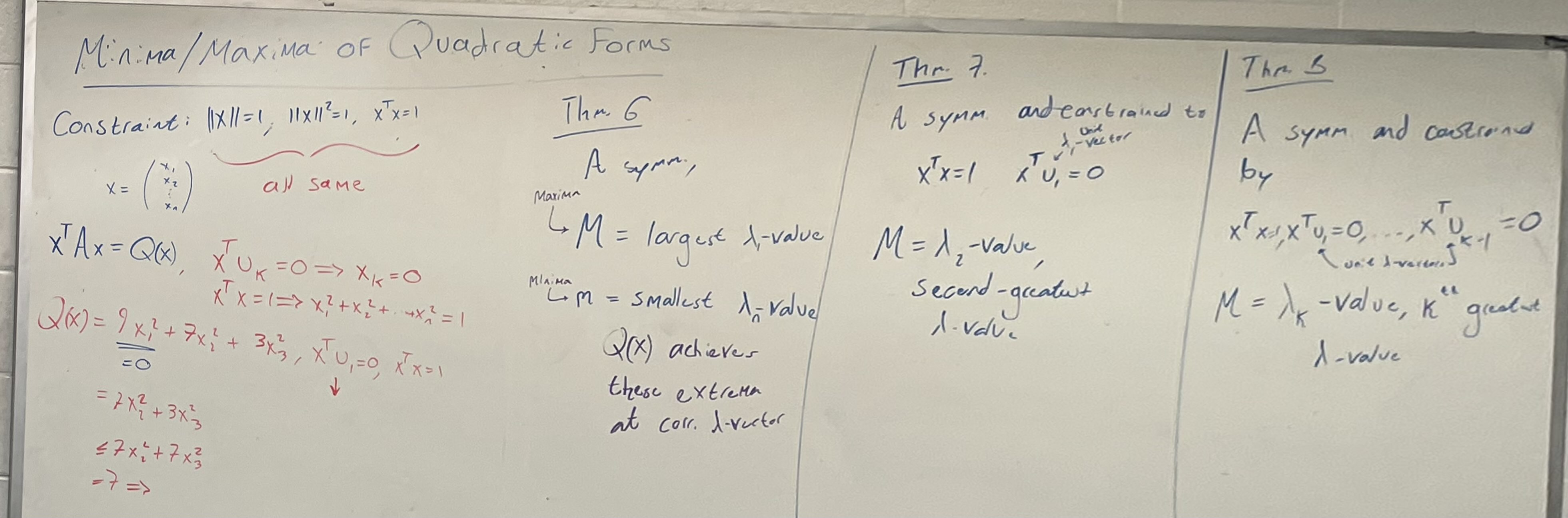
Constrained Optimization
Q: When for the first greatest eigenvalue, and the remaining ones were -2, and 0, the next maximum was -2 instead of 0?
Link to original

Singular Value Decomposition
https://www.youtube.com/watch?v=vSczTbgc8Rc

Applications

If A is a invertible square matrix then the condition number is the largest singular value divided by the smallest singular value

Condition number describes the sensitivity of a solution to Ax = b to errors in A

A problem with a low condition number is said to be well-conditioned, while a problem with a high condition number is said to be ill-conditioned

Describe difficulty in computing inverse

Chaos: small change in input results in massive change in output

Can use SVD to talk about rkA, ColA, RowA, NulA, , etc.

rkA = rk

ColA = U columns through dim A

bc

Col A perp = U columns after dim A

by def

Nul A = V columns that correspond to the free columns of U

Process

and are square, guaranteed.

Singular values:

Construct using the singular values. has the same shape as , with a diagonal matrix of the singular values in the top left corner

V = matrix of eigenvectors of

Compute an orthonormal basis for Col A: use for dim

Afterwhich, extend and fill up the remaining orthonormal basis

Option A: Rawdog itthink about it, so to speak

Option B: Gram-Schmidt Process

Option C: Use

Construct the columns of with the vectors

Note: for U you can also get it via the V process but with , for eigenvalue 0, find eigenvector

V and U are orthogonal btw, and they have dimensions of and

where , are the columns of and
Link to original

Explorer

Linear Algebra

Vectors and Vector Spaces

Vector Space

Vector Space Element

Axioms

Vector

Operations

Addition

Subtraction

Scalar Multiplication

Magnitude

Dot Product

Cross Product

Subspaces of

Subspace

Four Fundamental Subspaces

Columnspace

Rowspace

Nullspace

Basis

Dimension

Examples

Basis Theorem

Rank

Nullity

Fundamental Theorem of Linear Algebra

Invertibility Theorem

Determinant

Determinant Laws

Determinant Post Row Operations

Cofactor Expansion

Eigenstuff

Eigenvectors and Eigenvalues

Eigenvector

Eigenvalue

Defective

Neutral Eigenvalue

Eigenspace

Characteristic Equation

Characteristic Polynomial

Algebraic Multiplicity

Geometric Multiplicity

Similar

Systems of Linear Equations

Linear System

Representation

Linear Equation

Row Reduction

Row Operation

Row Operation

Consistent

Theorem for Consistency

Row Equivalent

Row Equivalent

Echelon Form

Echelon Form

Pivot

Free Variable

Vector Equations

Vector Equation

Real Number

Linear Combination

Span

Homogenous

Homogenous System

Homogenous System

Homogenous Differential Equation

Homogeneous Differential Equation

Linear Independence

Linear Independence

Geometric Interpretation

Linear Dependence

Intro to Linear Transformations

Linear Transformation

1-1

Injective

Onto

Surjective

Bijective