Digital Signal Processing

Digital Signal Processing is Signal Processing in the digital context, where you process Digital Signals.

Foundations

Signals

Signal

A signal is a way of carrying information from one place to another.

The Domain of a signal is almost always time. The Codomain is usually some kind of measure of amplitude, whether it be decibels, voltage, etc. An exception to the rule of thumb are inputs involving both space and time, such as sensor data from a satellite or a waymo or something, where the domain is spatiotemporal rather than just temporal, consisting of coordinates and time, and the codomain is some kind of multidimensional representation of color, usually RGBA, rather than a single scalar.

Levels of Discretization

Analog Signal

Analog Signal

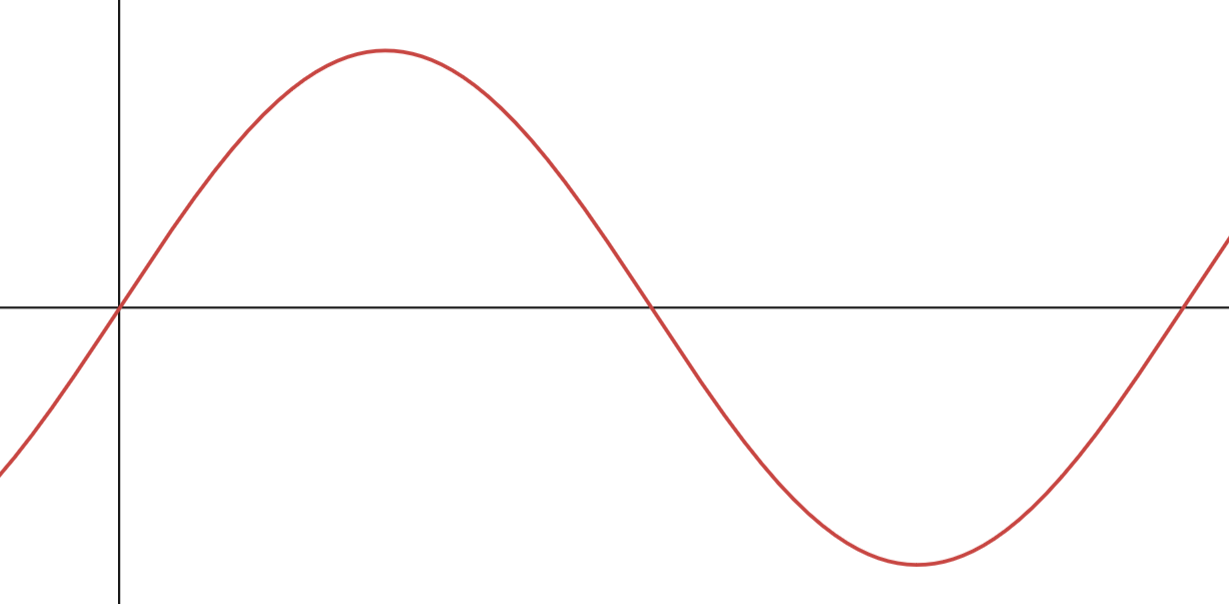
An analog signal is a Continuous wave. It is typically denoted as $x(t)$, where $x$ is the function of the wave and $t$ is time.

An example of an analog signal is sound; imagine a guitar string vibrating at an 440 Hz A. Not only is the string a continuous wave, but the compression waves it imparts onto the air, the sound, are also continuous waves.

Link to original

Discrete-Time Signal

Discrete-Time Signal

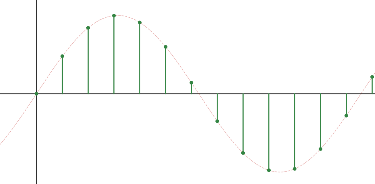
A discrete-time signal is the result of Sampling a subset of the domain of an Analog Signal, creating a new signal where the Domain is discrete, while the Codomain remains Continuous. It is typically denoted as $x[n]$, where $x$ is the function of the signal, and $n$ is the index.

An example of a discrete-time signal is within the process of digitally recording a guitar. While a microphone can hear any pitch, it can not convey every instant of a sound to a computer. Therefore, a broker responsible for converting the analog signal of the microphone into something the computer can understand is required. A Analog-to-Digital Converter decides on a certain sampling rate at which to note what the microphone hears at that moment so that it can eventually send a finite amount of information to the computer. At a certain stage within the converter, the signal is represented with discrete time, but the codomain is still continuous.

Link to original

Digital Signal

Digital Signal

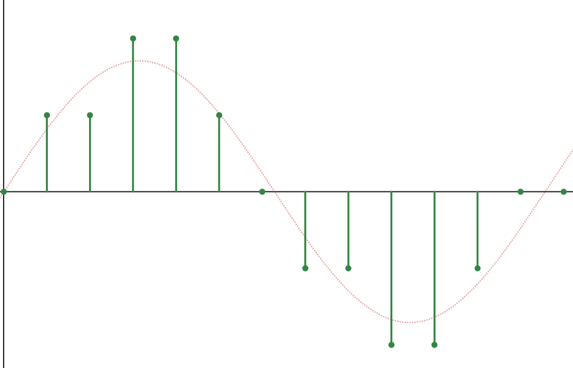
A digital signal is the result of Quantizing the values of the codomain of a Discrete-Time Signal, creating a new signal where both the Domain and Codomain are discrete. It is typically can be denoted as $x[n]$, where $x$ is the function of the signal, and $n$ is the index. It can also be denoted as $\hat{x}[n]$ or $x_q[n]$ to distinguish it from its discrete-time counterpart, and to show that it has been quantized.

An example of a digital signal would be the final steps of the Analog-to-Digital Converter before it sends the final digital signal to the computer; it has to represent that signal in binary. Any means of representing all continuous values with finite digits of precision will lead to loss, so regardless of if you choose IEEE 754 Doubles, or some kind of integer, you will be performing some level Quantization to the signal. The result is a signal with both discrete time and amplitude.

Link to original

Signal Transformations

Signals can be scaled, shifted, and flipped. They are subject to all of the typical Linear Transformations that maintain the validity of the Function. That is, not rotations, as they can break the vertical line test.

Signal Parity

Any signal can be uniquely decomposed into the sum of an Even Signal and an Odd Signal, by the Even-Odd Decomposition Property.

Even Signal

An even signal is a signal whose underlying function is an Even Function

Odd Signal

An odd signal is a signal whose underlying function is an Odd Function

Special Signals

Discrete Delta Function

The Kronecker Delta Function but it is a Discrete-Time Signal.

Impulse Representation

Impulse

In Discrete-Time land, an Impulse $\delta [n]$ is a Signal that is a discrete Kronecker Delta Function

$$\begin{array}{r}\delta [n]=\{\begin{array}{ll}1,& n=0\\ 0,& n\ne 0\end{array}\\ \\ \delta [n]=[1,\vec{0}]\end{array}$$

Note that for Convolutions, this unit impulse is like the Identity

$$x[n]\ast \delta [n]=x[n]$$

Similar to the Step Function, you can scale or shift the delta function. Furthermore, you can compose these scaled and shifted delta functions to create ANY given signal.

For example, $x[n]$ is a signal that goes: 1, 2, 3.

$$x[n]=1\cdot \delta [n]+2\cdot \delta [n-1]+3\cdot \delta [n-2]$$Link to original

Sifting Property

Sifting Property

You can also use the delta function to “sift” out the output of a signal at a given $n_0$

$$x[n_0]=\sum _{n=-\infty }^{\infty }x[n]\delta [n-n_0]$$

This can be used for either constructing or deconstructing a signal.

Link to original

Discrete Step Function

The Heaviside Step Function but it is a Discrete-Time Signal.

Moving between the Step and Delta Functions

$$\begin{array}{rl}\delta [n]& =u[n]-u[n-1]\\ u[n]& =\sum _{k=-\infty }^n\delta [k]\end{array}$$

Periodicity

A signal is periodic if it repeats its pattern exactly over and over again at regular, predictable intervals.

A discrete signal $x[n]$ is periodic iff $\exists N\in {\mathbb{Z}}^{+},s.t.x[n+N]=x[n],\forall n\in \mathbb{Z}$

This is important because a function in continuous-time can be periodic, but if that period is not an integer, then it is not neccessarily periodic in discrete-time! Alternatively, if a function’s period is an integer, it will be period in both continuous, and discrete-time (assuming step = 1).

Link to original

Sampling

Circular transclusion detected: Computer-Science/Computational-Science/DigitalSignalProcessing/Sampling

Band

Band

band (short for Frequency band) refers to a continuous, defined range of frequencies between an upper and lower limit.

Band Types

Passband

A Frequency Band referring to the range of frequencies that are allowed to pass through a Filter

Link to original

Stopband

A Frequency Band referring to the range of frequencies that a filter attenuates.

Link to original

Transition Band

A Frequency Band referring to the narrow range of frequencies between the Passband and the Stopband, i.e. the transition range.

Link to original

Guard Band

A Frequency Band referring to the range of frequencies in between two active bands left intentionionally vacant, acting as a guard or buffer zone, in order to mitigate cross-talk.

Link to original

Bandwidth

Bandwidth

Bandwidth is the width of a Band, the difference between the upper and lower frequency limits of a signal or channel. You can also think of it as the spread of a Signal’s Frequency Spectrum in the frequency domain.

$$B=f_{high}-f_{low}$$

Shannon’s Channel Capacity Theorem

Shannon's Channel Capacity Theorem

The maximum Data Rate $C$ achievable over a channel of Bandwidth $B$ with a given Signal-to-Noise Ratio is:

$$\begin{array}{rl}C& =B{\log }_2(1+\text{SNR})\\ C& \propto B\end{array}$$Link to original

Link to original

Link to original

Windowing

Windowing

Windowing is when you multiply a Window Function by a Signal to extract a finite “window” of it.

Window Function

A window function is the function you multiply by the function of the signal to yield a “window” of the signal.

Rectangle Window

When you use rect as the window function, you get an exact subsection of the original signal. However, you also get Spectral Leakage due to the abrupt cutoff of the function. The other window functions solve this by tapering the product to zero by the edges.

Hann Window

Hann window uses a raised cosine shape that tapers smoothly to exactly zero at the edges to reduce Spectral Leakage.

$$w[n]=0.5\left(1-\cos \left(\frac{2\pi n}{N-1}\right)\right)$$

Hamming Window

The Hamming window is a slight modification of the Hann Window optimized to minimize the height of the maximum side-lobe. Instead of tapering all the way to zero, it tapers to a small non-zero value.

$$w[n]=0.54-0.46\cos \left(\frac{2\pi n}{N-1}\right)$$

Blackman Window

The Blackman Window is the smoother version of the Hann Window, achieving this smoother taper through an additional cosine term.

$$w[n]=0.42-0.5\cos \left(\frac{2\pi n}{N-1}\right)+0.08\cos \left(\frac{4\pi n}{N-1}\right)$$Link to original

Quantization

Quantization

In Digital Signal Processing, Quantization is the discretization of the Codomain of a Discrete-Time Signal, making a it a true Digital Signal.

Link to original

Transforms

Fourier Transform

Fourier Transform

An approach for computing what frequencies are present in a Wave, in particular the Frequency Spectrum, entirely from its dependence on time. Allows us to transform a function between time an frequency domains. Allows us to quantitivatively define the Frequency Spectrum of a Wave A Gaussian’s transform is another Gaussian.

• Frequency is conjugate to time
• Spatial frequency is conjugate to position Anytime the Fourier Transform is involved, so is the Scale Theorem, and the Uncertainty Principle

Equation

$$F(\omega )={\int }_{-\infty }^{\infty }f(t)e^{-i\omega t}dt$$

• Where $F(\omega )$ is called the Fourier Transform of $f(t)$, containing equivalent information to that in $f(t)$
• $f(t)$ lives in the time domain
• $F(\omega )$ lives in the frequency domain

Fourier Transform with respect to space

A spatial fourier transform. Spatial frequency $k$ is the conjugate of position $x$.

$$F(k)\equiv {\int }_{-\infty }^{\infty }f(x)\exp (-ikx)dx$$

Derivation from Fourier Series

Let $F(m)\equiv {\mathbb{E}}_m-i{\mathbb{O}}_m$ where these values are defined in Even Function and Odd Function and also Fourier Series

$$\begin{array}{r}\\ F(m)\equiv {\mathbb{E}}_m-i{\mathbb{O}}_m=\\ \int f(t)\cos (mt)dt-i\int f(t)\sin (mt)dt=\\ \int f(t)e^{-imt}dt\end{array}$$

Allow t to range from $-\infty$ to $\infty$, $m$ to be continuous Frequency $\omega$, i.e. for a continuous range of frequencies

$$F(\omega )={\int }_{-\infty }^{\infty }f(t)e^{-i\omega t}dt$$

Fourier Transform of the Complex Conjugate of a Function

$$\mathcal{F}(f^{\ast }(t))=F^{\ast }(\omega )=F^{\ast }(-\omega )$$

Fourier Transform of the Sum of Two Functions

$$\mathcal{F}(a\cdot f(t)+b\cdot g(t))=a\mathcal{F}(f(t))+b\mathcal{F}(g(t))$$

Inverse Equation

$$f(t)=\frac{1}{2\pi }{\int }_{-\infty }^{\infty }F(\omega )e^{-i\omega t}d\omega$$

Derivation from Fourier Series

Note that the $i$ gets factored in for consistency with the above derivation.

$$\begin{array}{r}f(t)=\\ \mathbb{E}(t)+\mathbb{O}(t)=\\ \frac{1}{\pi }\sum _{m=0}^{\infty }{\mathbb{E}}_m\cos (mt)+\frac{1}{\pi }\sum _{m=0}^{\infty }{\mathbb{O}}_m\sin (mt)=\\ \frac{1}{2}\left(\frac{1}{\pi }{\int }_{-\infty }^{\infty }{\mathbb{E}}_m\cos (mt)dt+\frac{1}{\pi }{\int }_{-\infty }^{\infty }{\mathbb{O}}_m\sin (mt)dt\right)=\\ \frac{1}{2}\left(\frac{1}{\pi }{\int }_{-\infty }^{\infty }\left({\mathbb{E}}_m\cos (mt)+i{\mathbb{O}}_m\sin (mt)\right)dt\right)=\\ \frac{1}{2}\left(\frac{1}{\pi }{\int }_{-\infty }^{\infty }\left(F(\omega )\cos (mt)+iF(\omega )\sin (mt)\right)dt\right)=\\ \frac{1}{2}\left(\frac{1}{\pi }{\int }_{-\infty }^{\infty }F(\omega )e^{-i\omega t}dt\right)=\\ \frac{1}{2\pi }{\int }_{-\infty }^{\infty }F(\omega )e^{-i\omega t}d\omega \end{array}$$

Fourier Tranform with respect to space

$$f(x)=\frac{1}{2\pi }{\int }_{-\infty }^{\infty }F(k)\exp (ikx)dk$$

Notation

If original function lowercase, use above notation

• $f(t)$ for the function
• $F(\omega )$ for the transform If the original function is uppercase:
• $E(t)$ for the function, arbitrarily
• For the transform
  • $\mathcal{F}\left(E(t)\right)$
  • $\tilde{E}(\omega )$

Examples

Find $\mathcal{F}(\text{rect}(t))$

$$\begin{array}{r}\\ F(\omega )={\int }_{-0.5}^{0.5}\exp (-i\omega t)dt=\\ \frac{1}{-i\omega }(\exp (-i\omega t){)}_{-0.5}^{0.5}=\\ \frac{1}{-i\omega }\left(\exp \left(-\frac{i\omega }{2}\right)-\exp \left(\frac{i\omega }{2}\right)\right)=\\ \frac{1}{\frac{\omega }{2}}\frac{\exp \left(\frac{i\omega }{2}\right)-\exp \left(-\frac{i\omega }{2}\right)}{2i}=\\ \frac{\sin \left(\frac{w}{2}\right)}{\frac{\omega }{2}}\equiv \\ \text{sinc}\left(\frac{\omega }{2}\right)\end{array}$$

See sinc for more info

Theorems

Scale Theorem

Scale Theorem

Fourier Transform of a scaled function $f\left(\frac{t}{a}\right)$

$$\mathcal{F}\left(f\left(\frac{t}{a}\right)\right)=|a|F(a\omega )$$

• $a\in \mathbb{C}$ is allowed
• Implies that the shorter the Pulse of a Wave, the broader the Frequency Spectrum
• Implies Uncertainty Principle

Link to original

Modulation Theorem

Modulation Theorem

$$\mathcal{F}(E(t)\cos ({\omega }_{0}t))=\frac{1}{2}\tilde{E}(\omega -{\omega }_0)+\frac{1}{2}\tilde{E}(\omega +{\omega }_0)$$Link to original

Shift Theorem

Shift Theorem

The Fourier Transform of a shifted function $f(t-\tau )$

$$\mathcal{F}(f(t-\tau ))=\exp (-i\omega t)F(\omega )$$Link to original

Convolution Theorem

Convolution Theorem

The convolution theorem states that the Fourier Transform of a Convolution of two functions is equal to the product of their Fourier transforms.

$$\mathcal{F}\{x[n]\ast h[n]\}=X(e^{jw})\cdot H(e^{jw})$$Link to original

2D Fourier Transform

2D Fourier Transform

$$\begin{array}{r}{\mathcal{F}}^{(2)}(f(x,y))=\\ F(k_x,k_y)=\\ \int \int f(x,y)\exp (-i(k_{x}x+k_{y}y))dxdy\end{array}$$

See Also

• Fourier Transform
• K Vector
• Wave
• Fraunhofer Diffraction

Link to original

Link to original

Discrete Fourier Transform

Discrete Fourier Transform

$$X[k]=\sum _{n=0}^{N-1}x[n]\cdot {\omega }_N^{nk}$$

• where ${\omega }_N=\exp \left(-\frac{2i\pi }{N}\right)$, called the “Nth root of unity”
  • Nth roots of unity is the related concept of the complex unit circle being split up equally into $N$ sectors, where integer powers of ${\omega }_N$ walk the circle
  • ${\omega }_N^{2a}={\omega }_{N/2}^a,a\in \mathbb{N}$
• where $N$ is the number of samples in the DT signal $x$
• where $k$ is the $k^{\text{th}}$ frequency bin, representing an area of frequencies in the frequency domain centered around $\frac{k{f}_s}{N}$, where $f_s$ is the Sampling Frequency
  • the spacing between bins is $\Delta f=\frac{f_s}{N}$, called the bin width
• where $X$ is a Complex Number
• where the input is assumed to be periodic with period $N$

Time Complexity

The Time Complexity of calculating the Discrete Fourier Transform as a Matrix product or by equivalently calculating each Dot Product per $k$ without matrices is $O(n^2)$, where the DFT Matrix $W$ is a Square Matrix

Use Cases of DFT

• FFT is most commonly used
• Approximate Derivatives $\to$ Solve PDEs
• Denoise Data
• Data Analysis
• Compression
  • Audio Compression
  • Image Compression
  • Wavelet Transform

Matrix Discrete Fourier Transform

$$\left[\begin{array}{c}X[0]\\ X[1]\\ X[2]\\ ⋮\\ X[N-1]\end{array}\right]=\left[\begin{array}{ccccc}1& 1& 1& \cdots & 1\\ 1& {\omega }_N& {\omega }_N^2& \cdots & {\omega }_N^{N-1}\\ 1& {\omega }_N^2& {\omega }_N^4& \cdots & {\omega }_N^{2(N-1)}\\ ⋮& ⋮& ⋮& \ddots & ⋮\\ 1& {\omega }_N^{N-1}& {\omega }_N^{2(N-1)}& \cdots & {\omega }_N^{(N-1{)}^2}\end{array}\right]\left[\begin{array}{c}x[0]\\ x[1]\\ x[2]\\ ⋮\\ x[N-1]\end{array}\right]$$ $$\begin{array}{rl}\text{Let }W& \in {\mathbb{C}}^{N\times N}s.t.W_{i,j}={\omega }_N^{ij}\\ \vec{X}& =W\vec{x}\end{array}$$

• where $W$ is called the “DFT Matrix”

Inverse Discrete Fourier Transform

$$x[n]=\frac{1}{N}\sum _{k=0}^{N-1}X[k]\cdot {\omega }_N^{-nk}$$

Power Spectrum

Power Spectrum

The power spectrum is the distribution of Signal Power across frequency, computed by taking the squared magnitude of each DFT bin $k$:

$$P[k]=|X[k]{|}^2=I[k{]}^2+Q[k{]}^2$$

It discards phase information and retains only energy per frequency bin. The primary domain for signal detection; bins whose power exceeds the local noise floor are declared detections.

Link to original

FFT Shift

FFT Shift

The FFT Shift post-processes the output frequency graph of the FFT and centers 0 in the middle of the array, rather than at the beginning, making it easier to interpret. By default frequencies of zero are on the left, then positives, then negatives.

$$[k_0,{\vec{k}}_{+},{\vec{k}}_{-}]\to [{\vec{k}}_{-},k_0,{\vec{k}}_{+}]$$Link to original

Link to original

Fast Fourier Transform

Fast Fourier Transform

The Fast Fourier Transform (FFT) is the de facto Algorithm for calculating the Discrete Fourier Transform, that reduces the Time Complexity of the computation to $O(n\log n)$, whereas a regular matrix multiplication is $O(n^2)$. There are many different implementations of the FFT.

Time Complexity

The Time Complexity of the FFT algorithm is $O(n\log n)$, whereas the naive DFT algorithm is $O(n^2)$.

The TLDR on the intuition for the time complexity is that we can split up the original DFT into subproblems until we have $O(\log n)$ subproblems that each take $O(n)$ to compute. Hence the time complexity is $O(n\log n)$.

• $N^2\leftarrow$ in the original expression, we iterate $N$ to sum, $N$ times
• $2\cdot {\left(\frac{N}{2}\right)}^2=\frac{N^2}{2}\leftarrow$ we iterate $N/2$ to sum, $N/2$ times, and we do that twice
• $4\cdot {\left(\frac{N}{4}\right)}^2=\frac{N^2}{4}\leftarrow$ the second level of recursion
• $N\cdot {\left(\frac{N}{N}\right)}^2=\frac{N^2}{N}=N\leftarrow$ the last level of recursion

Cooley-Tukey FFT

Radix-2 FFT

Radix-2 FFT is a FFT implementation that requires $N$ is a power of $2$

Radix-2 Decimation in Time FFT

For DIT, you split by the index (n) by parity. Hence “decimation in time”.

Start with the initial DFT equation

$$X[k]=\sum _{n=0}^{N-1}x[n]\cdot {\omega }_N^{nk}$$

Split the odd and even indices into two different sums

$$X[k]=\sum _{m=0}^{N/2-1}x[2m]\cdot {\omega }_N^{(2m)k}+\sum _{m=0}^{N/2-1}x[2m+1]\cdot {\omega }_N^{(2m+1)k}$$

Factor out a ${\omega }_N^k$ from the odd sum

$$X[k]=\sum _{m=0}^{N/2-1}x[2m]\cdot {\omega }_N^{(2m)k}+{\omega }_N^k\sum _{m=0}^{N/2-1}x[2m+1]\cdot {\omega }_N^{(2m)k}$$

Rewrite the the subproblem DFTs as the odd indices subproblem and the even indices subproblem. Each of these subproblem DFTs are only half the length as the original problem, so while $k$ was originally valid beyond $\frac{N}{2}$ for $X[k]$, it must now be within the half range to accomodate $X_O[k]$ and $X_E[k]$.

$$X[k]=X_E[k]+{\omega }_N^k\cdot X_O[k]\text{for }0\le k<\frac{N}{2}$$

In order to calculate the full DFT, we have to get the values of $X[k]$ for $\frac{N}{2}\le k<N$, which we can do this by shifting the result we just got.

$$X\left[k+\frac{N}{2}\right]=X_E\left[k+\frac{N}{2}\right]+{\omega }_N^{k+N/2}\cdot X_O\left[k+\frac{N}{2}\right]$$

Simplify subproblem DFTs using periodicity rules: period of $\frac{N}{2}$ sample DFT is $\frac{N}{2}$

$$X\left[k+\frac{N}{2}\right]=X_E\left[k\right]+{\omega }_N^{k+N/2}\cdot X_O\left[k\right]$$

Using ${\omega }_N^{k+N/2}={\omega }_N^k\cdot {\omega }_N^{N/2}=-{\omega }_N^k$ , where ${\omega }_N^{N/2}=e^{-i\frac{2\pi }{N}\cdot N/2}=e^{-\pi i}=-1$

$$X\left[k+\frac{N}{2}\right]=X_E[k]-{\omega }_N^k\cdot X_O[k]\text{for }0\le k<\frac{N}{2}$$

Therefore now we have the capability of calculating $X[k]$ for all relevant $k$ using the combination of these two, where the upper range $k$ use the bottom and the lower range use the top. The resulting process is called the Butterfly Operation, allowing us to convert an $N$-point DFT problem into two $N/2$-point DFT problems.

$$\begin{array}{rl}X[k]& =X_E[k]+{\omega }_N^k\cdot X_O[k]\\ X\left[k+\frac{N}{2}\right]& =X_E[k]-{\omega }_N^k\cdot X_O[k]\\ & \text{for }0\le k<\frac{N}{2}\end{array}$$

• $N^2\leftarrow$ in the original expression, we iterate $N$ to sum, $N$ times
• $2\cdot {\left(\frac{N}{2}\right)}^2=\frac{N^2}{2}\leftarrow$ we iterate $N/2$ to sum, $N/2$ times, and we do that twice
• $4\cdot {\left(\frac{N}{4}\right)}^2=\frac{N^2}{4}\leftarrow$ the second level of recursion
• $N\cdot {\left(\frac{N}{N}\right)}^2=\frac{N^2}{N}=N\leftarrow$ the last level of recursion

We have already shown the first level of recursion. If we keep on recursing until each subvector is of length 1, then it only cost $N$ to calculate that DFT subproblem. It takes $\log n$ recurses to get to the base case.

Radix-2 Decimation in Frequency FFT

For DIF, you split the frequencies (k) by parity. Hence “decimation in frequency”.

Good-Thomas FFT

Also known as the Prime-Factor Algorithm FFT, you break $N$ into factors that are strictly coprime, meaning that their GCD = 1. This one isn’t as relevant to computation though, so we just mention it. Radix 2, is the main one for computation because computers love 2.

​Link to original

Z Transform

Z Transform

todo

Link to original

Digital Filtering

Filter

A medium through which a Signal propogates that alters its amplitude, frequency, or phase characteristics, in order to pass desired characteristics while attenuating undesired ones.

Basic Filter Types

Low-Pass Filter

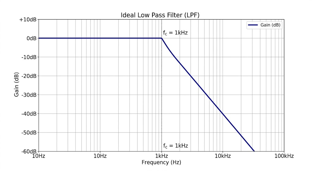
Low-Pass Filter

A Filter that only passes low frequencies.

Link to original

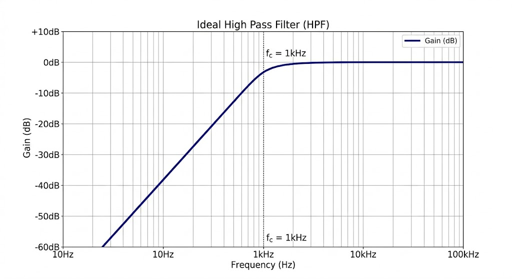
High-Pass Filter

High-Pass Filter

A Filter that only passes highest frequencies.

Link to original

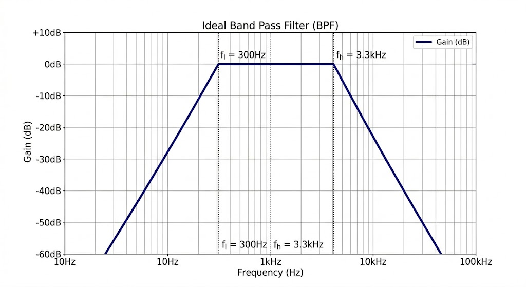
Band-Pass Filter

Band-Pass Filter

A Filter that only passes a specific Frequency Band

Link to original

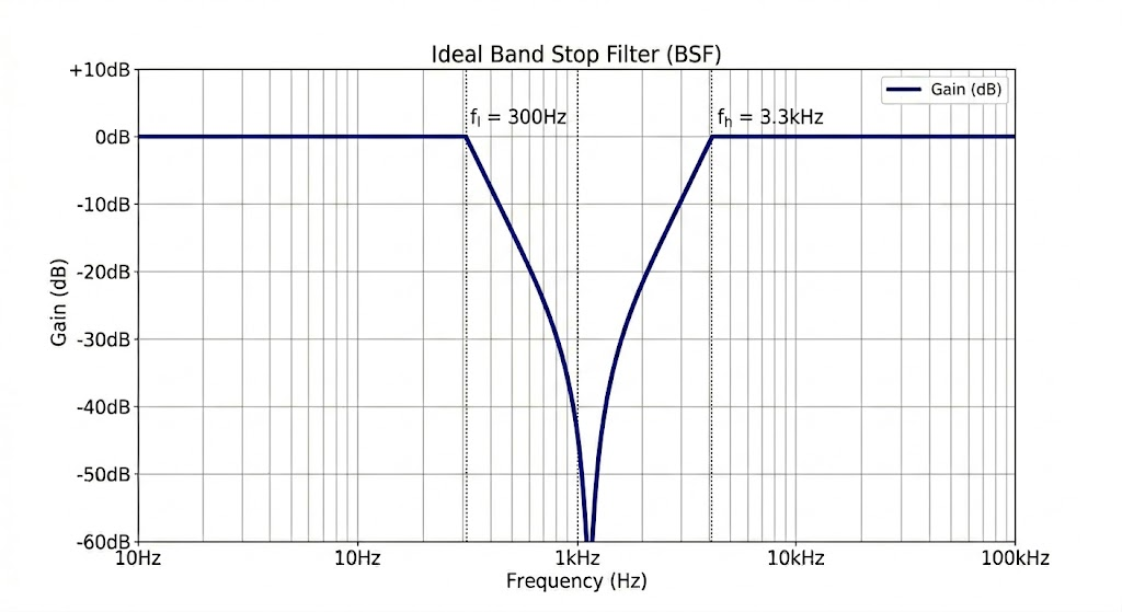
Band-Stop Filter

Band-Stop Filter

A Filter that passes every frequency except for a specific Frequency Band

Link to original

Impulse Response Filters

Impulse Response

Impulse Response

In Digital Signal Processing, Impulse Response is the output of a system when it is subjected to an Impulse.

For example, the impulse response of a reverb filter would continuously fade the volume from the impulse over time. An echo filter would periodically repeat the impulse, while fading the volume over time. A gain filter would have no temporal effect like the aforementioned.

$h[n]$ is used to denote the impulse response of a system where

$$h[n]=T\{\delta [n]\}$$

Impulse response is important in DSP because if a system in a Linear Time-Invariant System, then knowing $h[n]$ means you know everything about the system, where $T$ is the system.

$$T\{x[n]\}=x[n]\ast h[n]$$Link to original

Finite Impulse Response Filter

Finite Impulse Response Filter

A Finite Impulse Response Filter is a Linear Time-Invariant System Filter whose Impulse Response eventually becomes zero, or in other words, the duration of response to the Impulse Signal is finite. This property is due to such filters being Feed-Forward.

$$\begin{array}{c}\mathcal{H}:{\mathbb{R}}^{\mathbb{Z}}\times \mathbb{Z}\to \mathbb{R}\\ \mathcal{H}(x,n)=y[n]\\ y[n]={\sum }_{k=0}^M{b}_k\cdot x[n-k]\end{array}$$

• Because FIR Filters are Feed-Forward, they are massively more parallel and belong in CUDA algorithms on the GPU, whereas IIR Filter is inherently iterative and thus is better suited for the CPU

Z Transform

$$\begin{array}{rl}H(z)& =\sum _{k=0}^M{b}_k\cdot z^{-k}\\ & =b_0\prod _{k=1}^M(1-c_k{z}^{-1})\\ & \end{array}$$

• See Z Transform

Impulse Response

$$h[n]=\{\begin{array}{ll}{b}_n& 0\le n\le M\\ 0& \text{else}\end{array}$$

• See Impulse Response

Link to original

Infinite Impulse Response Filter

Infinite Impulse Response Filter

An Infinite Impulse Response Filter is a Linear Time-Invariant System Filter whose Impulse Response never becomes zero, or in other words, the duration of response to the Impulse Signal is infinite. This property is due to such filters being recursively defined, i.e. having Feedback.

$$\begin{array}{c}\mathcal{H}:{\mathbb{R}}^{\mathbb{Z}}\times {\mathbb{R}}^{\mathbb{Z}}\times \mathbb{Z}\to \mathbb{R}\\ \mathcal{H}(x,y,n)=y[n]\\ y[n]={\sum }_{k=0}^M{b}_{k}x[n-k]-{\sum }_{k=1}^N{a}_k\cdot y[n-k]\\ \end{array}$$

• Because IIR Filters are Feed-Back
  • They are is inherently iterative and thus better suited for the CPU, rather than GPU which is where FIR belongs
  • Caching becomes even more important
  • They can be Divergent, which can lead to Overflow. Thus, Stability needs to be considered

Z Transform

$$\begin{array}{rl}H(z)& =\frac{{\sum }_{k=0}^M{b}_k{z}^{-k}}{{\sum }_{k=0}^N{a}_k{z}^{-k}},a_0=1\\ & =\frac{b_0{\prod }_{k=1}^M(1-c_k{z}^{-1})}{{\prod }_{k=1}^N(1-d_k{z}^{-1})}\\ & \end{array}$$

• See Z Transform

Divergence

For a system with poles $d_k$

• Asymptotically Stable $⟺\forall k,|d_k|<1$
• Marginally Stable $⟺\forall k,|d_k|\le 1$ and all poles with $|d_k|=1$ are Algebraic Multiplicity of 1
• Unstable $⟺\exists k,|d_k|>1$ or $\exists k,|d_k|=1$ with Algebraic Multiplicity greater than 1

Impulse Response

$$h[n]=\sum _{k=1}^N{A}_k(d_k{)}^{n}u[n]$$

• See Impulse Response

Link to original

Link to original

Modulation

Modulation

Modulation is the process of embuing a signal inside a Carrier Wave in order to convey information through that wave.

Analog Modulation

Amplitude Modulation (AM)

Amplitude Modulation

todo

Link to original

Frequency Modulation (FM)

Frequency Modulation

todo

Link to original

Phase Modulation (PM)

Phase Modulation

todo

Link to original

Digital Modulation

Phase Shift Keying (PSK)

Phase Shift Keying

todo

Link to original

Frequency Shift Keying (FSK)

Frequency Shift Keying

todo

Link to original

Quadrature Amplitude Modulation (QAM)

Quadrature Amplitude Modulation

todo

Link to original

Orthogonal Frequency Division Multiplexing (OFDM)

Orthogonal Frequency Division Multiplexing

todo

Link to original

Link to original

Estimation & Modeling

Spectrum Estimation

todo

Parametric Signal Modeling

todo

Kalman Filters

Kalman Filter

todo

Extended Kalman Filter

todo

Miscellaneous

Beamforming

todo

Double Buffering

todo