Statistics

Statistics is the study of predicting Populations from Samples

Statistic

Statistic

A Statistic is a scalar feature extracted from a Sample that represents it in some way. As opposed to Parameter.

$$T:X_{\mathrm{1..}n}\in \text{RV}\to \mathbb{R}$$

Sample Statistic

• Sample Mean $\overline{X}=\frac{\sum X}{n}$
• Sample Median: Middle entry in Sample
• Sample Mode: Most occurences in Sample
• Sample Variance $S^2=\frac{\sum (X-\overline{X}{)}^2}{n-1}$
• Sample Standard Deviation $S$
• Sample Proportion $\hat{p}=\frac{x}{n}$

Centrality Features

• Sample Mean, Median, Mode. Median is best.

Spread Features

• Sample Range $\max X-\min X$
• Sample Variance, Standard Deviation
• Percentile
• Quartile, Inter Quartile Range

Grouped Features

$$\overline{X}-\frac{1}{n}\sum _{j=1}^p{f}_j{x}_j{S}^2=\frac{1}{n-1}\left(\sum _{j=1}^p{f}_j{x}_j^2-n{x}^2\right)$$Link to original

In the real world, you don’t Parameters, so you have to approximate them with Statistics. In Statistics, our goal is to analyze population(s) without omnipotence.

Point Estimation

Point Estimation

A Point Estimator is a Statistic that is designed to estimate a Parameter.

• A regular statistic is just any feature from the data, whereas a Point Estimator specifically involves using the feature to predict the population parameter
• In order to evaluate how good a Point Estimator is, our goal is to minimize Mean Squared Error, i.e. both Bias and Variance. Minimizing MSE maximizes accuracy of the Point Estimator.
• In order to find a Point Estimator we can use techniques such as
  • Method of Moments
  • Maximum Likelihood Estimator

Bias

Bias is a measure of the expected difference between a Point Estimator and a Parameter. Imagine shooting arrows at a target. Bias refers to displacement of the center of the cluster from the bullseye.

$$\frac{\begin{array}{ccc}{X}_{\mathrm{1..}n}{\sim }^{iid}f(x;\theta )& T:{\mathbb{R}}^n\to \mathbb{R}& \hat{\theta }=T(X_{\mathrm{1..}n})\end{array}}{\text{Bias}(\hat{\theta })=E[\hat{\theta }]-\theta }$$

• where $T$ is a Statistic
• where $\theta$ is a Parameter of $X_{\mathrm{1..}n}$
• where $\hat{\theta }$ is a Point Estimator

Variance

Variance measures spread of a Point Estimator. Imagine shooting arrows at a target. Variance measures how spread out the arrows are from each other (and specifically not from the bullseye).

Point Estimation Features

• Standard Error $\sqrt{\text{Var}(\hat{\theta })}$
• Sample Mean $\overline{X}$
  • $E(\overline{X})=\mu$
  • $\text{Var}(\overline{X})=\frac{{\sigma }^2}{n}$
  • $S.E.=\frac{\sigma }{\sqrt{n}}$

Mean Squared Error

Mean Squared Error (MSE) measures how good a Point Estimator is. The lower the MSE, the more accurate a Point Estimator is, even if it does not minimize Bias.

$$\text{MSE}(\hat{\theta })=E[(\hat{\theta }-\theta {)}^2]=\text{Bias}(\hat{\theta }{)}^2+\text{Var}(\hat{\theta })$$

Finding a Point Estimator

Method of Moments

Method of Moments

In Point Estimation, we want to estimate parameters $\theta$ of an unknown population distribution using sample data. To do this, we borrow the concept of moments from physics.

In general, a moment is a weighted distance from an axis. The moment of force is torque, where the weight is force or literal weight. Imagine a flat seesaw at rest with weights distributed across it. The torque each weight applies is the product of x, the signed distance from the axis of rotation, and F, the force of the weight. The net torque, the sum of these individual torques.

$$\tau =xF{\tau }_{\text{net}}=\sum _i{x}_i{F}_i$$

Furthermore, instead of only indexing each occurence of a torque, we can alternatively create a function $f(x)$ that gives the force at every $x$, which allows us to write ${\tau }_{\text{net}}$ as a discrete or continuous sum over a domain $D$.

$$\begin{array}{rl}{\tau }_{\text{net}}& =\sum _{x\in D}x\cdot f(x)\text{or}{\int }_{D}x\cdot f(x)dx\\ & =\text{sum}x\cdot f(x)\end{array}$$

where the “sum” expression is shorthand for this summation regardless of whether $f(x)$ is discrete or continuous.

We can also reinterpret our $f(x)$ to be a PMF/PDF instead of a force function. You will recognize the moment equation above as Expected Value.

$$E[X]=\text{sum}xf(x)$$

We care about this $f(x)$ because it contains information about the hidden parameters of the population distribution that we are sampling from, including the parameter we want to estimate.

We define the kth order moment as the following, where k > 1 is used for systems of equations with greater than one unknown, to provide additional valid equations until we have a well-determined system of equations.

$$E[X^k]=\text{sum}{x}^{k}f(x)$$

Yep. It’s just literally just expected value. And when we use the higher degrees of k, it literally just adjusts the scale of the x axis (distance from the axis) from linear to quadratic to cubic to quartic, etc etc. Each new k value results in a new polynomially scaled version of the original distribution that gives a new equation that we can use to solve the system of equations that I am going to shortly introduce.

Notice how $E(X)=\text{fn}(\text{parameters})$

• $X\sim N\to E(X)=\mu$
• $X\sim \text{Pois}\to E(X)=\lambda$
• $X\sim \text{U}(a,b)\to E(X)=\frac{a+b}{2}$

Furthermore, we can also calculate sample moments, for k = 1 or above if needed.

$$\begin{array}{rl}{X}_{\mathrm{1..}n}{\sim }^{\text{iid}}f(x;n)& ⟹{\overline{X}}^k=\frac{1}{n}\sum _{i=1}^n{X}_i^k\\ & ⟹\overline{X}=\frac{1}{n}\sum _{i=1}^n{X}_i\end{array}$$

Using the following idea, we can estimate our parameters in the following way.

$$\overline{X}\approx E(X)=\text{fn}(\theta )⟹\overline{X}\approx \text{fn}(\theta )$$

Or if more than k = 1 is needed, the following is also applicable

$${\overline{X}}^k\approx E(X^k)=\text{fn}(\theta )⟹{\overline{X}}^k\approx \text{fn}(\theta )$$

Our system of equations is of the following form, where at least k = 1 is used, and where the range of k used is equal to the dimension of $\theta$

$$\begin{array}{c}{\overline{X}}^k=\frac{1}{n}{\sum }_{i=1}^n{X}_i^k\approx E(X^k)=\text{sum}{x}^{k}f(x)=\text{fn}(\theta )\\ ⟹{\overline{X}}^k\approx \text{fn}(\theta ),{\overline{X}}^k=\text{fn}(\hat{\theta })\end{array}$$

Examples

$X\sim N$

• Moment (k = 1): $E(X)=\mu$
• T ito $\theta$: $\overline{X}\approx \mu$ $\therefore \hat{\mu }=\overline{X}$

$X\sim \text{Pois}$

• Moment (k = 1): $E(X)=\lambda$
• T ito $\theta$: $\overline{X}\approx \lambda$ $\therefore \hat{\lambda }=\overline{X}$

$X\sim \text{Exp}(\lambda )$

• Moment (k = 1): $E(X)=\frac{1}{\lambda }$
• T ito $\theta$: $\overline{X}\approx \frac{1}{\lambda }$ $\therefore \hat{\lambda }=\frac{1}{\overline{X}}$

$X\sim U(0,\theta )$

• Moment (k = 1): $E(X)=\frac{\theta }{2}$
• T ito $\theta$: $\overline{X}\approx \frac{\theta }{2}$ $\therefore \hat{\theta }=2\overline{X}$

$X\sim U(a,b)$

• Moment (k = 1): $E(X)=\frac{a+b}{2}$
• Moment (k = 2): $E(X^2)=\frac{1}{3}(a^2+ab+b^2)$
• T ito $\theta$: $\overline{X}\approx \frac{a+b}{2},\overline{X^2}\approx \frac{1}{3}(a^2+ab+b^2)$ a + b &\approx 2\overline{X} \\ (a+b)^2 - ab &\approx 3\overline{X^2} \\ (2\overline{X})^2 - ab &\approx 3\overline{X^2} \\ ab &\approx 4\overline{X}^2 - 3\overline{X^2} \\ t^2 - (2\overline{X})t + (4\overline{X}^2 - 3\overline{X^2}) &\approx 0 \\ t &\approx \frac{2\overline{X} \pm \sqrt{(-2\overline{X})^2 - 4(1)(4\overline{X}^2 - 3\overline{X^2})}}{2} \\ t &\approx \overline{X} \pm \sqrt{3\left(\overline{X^2} - \overline{X}^2\right)} \\ a \approx \overline{X} - \sqrt{3\left(\overline{X^2} - \overline{X}^2\right)}, &\quad b \approx \overline{X} + \sqrt{3\left(\overline{X^2} - \overline{X}^2\right)} \end{align*}$$ $$\therefore\hat{a} = \overline{X} - \sqrt{3\left(\overline{X^2} - \overline{X}^2\right)}, \quad \hat{b} = \overline{X} + \sqrt{3\left(\overline{X^2} - \overline{X}^2\right)}$$

Link to original

Maximum Likelihood Estimator

For $X_{\mathrm{1..}n}{\sim }^{iid}f(x;\theta )$

We find MLE, which is the $\theta$ that maximizes the Likelihood Function $L$. $L$ is a scoring function that tells you how well your $\theta$ matches the observed data.

$$\begin{gathered} L(\theta )=\prod _{i=1}^{n}f(x_i) \\ \begin{array}{c}\max L=L(\text{MLE})\end{array} \end{gathered}$$

The trick for finding MLE

• Find $\ln (L(\theta ))$
• Find $\frac{\partial }{\partial \theta }\ln (L(\theta ))$
  • Recall $\frac{d}{dx}(\ln (f(x)))=\frac{f^{\prime }(x)}{f(x)}$
• Find where this equals 0
• Find which root is the max
• The $\max (\ln L)=\ln L$

Link to original

Confidence Intervals

Sample Distribution

Sample Distribution

A Sample Distribution is a Distribution that simply is the actual data of a single Sample.

Link to original

Sampling Distribution

Sampling Distribution

A Sampling Distribution is a Distribution of a particular Sample Statistic, sampled repeatedly from a Population. For example, a distribution of sample average heights.

Link to original

The Central Limit Theorem gives a Sample Mean Sampling Distribution where when $n$ is sufficiently large, the distribution is approximately a Z Distribution

Degree of Freedom

Degree of Freedom

Degrees of Freedom is a property of a Statistic or Point Estimator that describes how many variables are free to vary while maintaining the feature’s validity.

• For statistic/PE $T$ that is a Linear Transformation, dof = [Nullity|nullity]

Example

For example, a sample mean is a linear function of its inputs, because it is a sum of the RVs, all divided by a scalar. This is a linear transformation, as well.

$$\text{mean}(X_{\mathrm{1..}n})=\frac{\sum X_{\mathrm{1..}n}}{n}=\overline{X}$$

Due to this linearity, all of the inputs except for the last can be any value. If you allow the first $n-1$ RV to vary, then the $n^{\text{th}}$ RV is forced to a specific value.

$$X_n=n\overline{X}-\sum X_{\mathrm{1..}n-1}$$

Therefore, for sample mean, $\text{dof}=n-1$

Link to original

Chi Squared Distribution

Chi Squared Distribution

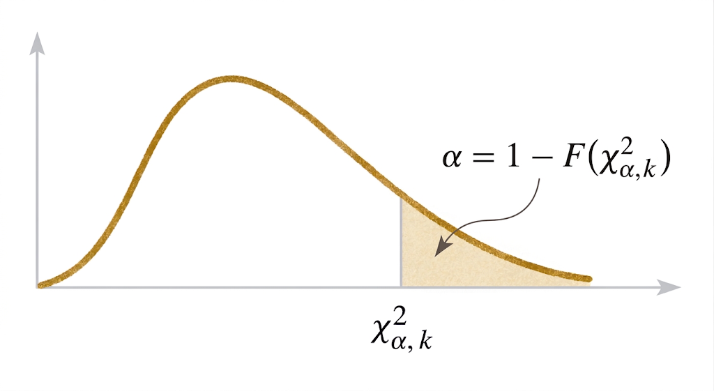
A ${\chi }^2$ Distribution is a kind of Sampling Distribution formed by combining iid squared Z Distributions through addition.

• ${\chi }^2$ shows up when we try to estimate Variance

$$\frac{Z_{\mathrm{1..}k}{\sim }^{\text{iid}}N(0,1)}{{\chi }_{(k)}^2\sim {\sum }_{i=1}^k{Z}_i^2}$$

• $E[Y]=k$
• $\text{Var}(Y)=2k$
• ${\chi }_{(1)}^2=Z^2$
• ${\chi }_{(2)}^2=\text{Exp}\left(\frac{1}{2}\right)$
• ${\chi }_{(\text{big})}^2\approx N$
• $k$ is Degree of Freedom

Additive Property

The sum of iid ${\chi }^2$ variables is also ${\chi }^2$

$$\frac{Y_{\mathrm{1..}n}{\sim }^{\text{indep}}{\chi }_{(k_i)}^2}{{\sum }_{i=1}^n{Y}_i\sim {\chi }_{\left({\sum }_{i=1}^n{k}_i\right)}^2}$$

Chi Squared Quantiles

If $Y\sim {\chi }_{(k)}^2$ then $(1-\alpha )$ quantile is denoted ${\chi }_{\alpha ,k}^2$

• where $P(Y>{\chi }_{\alpha ,k}^2)=1-F({\chi }_{\alpha ,k}^2)=\alpha$
• where $F$ is the ${\chi }^2$ CDF
• where $\alpha$ is type I error
• where $k$ is Degree of Freedom

Link to original

t distribution

Student's t distribution

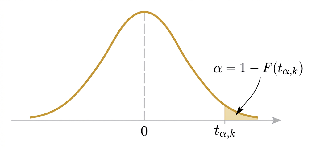
A Student’s $t$ Distribution is a kind of Sampling Distribution formed by combining a Z Distribution and Chi Squared Distribution in the following fashion

$$T\equiv \frac{Z}{\sqrt{{\chi }_{(k)}^2/k}}\sim t_{(k)}$$

• $t$ shows up when we try to estimate $\mu$ when the ${\sigma }^2$ is unknown.
• $t_{(k)}$ looks like $Z$ but with a fatter tail to account for the extra uncertainty of using $S^2$ instead of ${\sigma }^2$
• $t_{(k\to \infty )}=Z$
• $E[T]=0$
• $\text{Var}(T)=\frac{k}{k-2}\text{for }k>2$

Student’s t Quantiles

If $T\sim t_{(k)}$ then the $(1-\alpha )$ quantile is denoted $t_{\alpha ,k}$

• where $P(T>t_{\alpha ,k})=1-F(t_{\alpha ,k})=\alpha$
• where $F$ is the CDF
• where $\alpha$ is type I error
• where $k$ is Degree of Freedom
• where the distribution is symmetrical so $t_{1-\alpha ,k}=-t_{\alpha ,k}$

Link to original

F distribution

F distribution

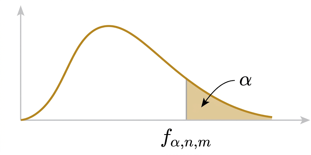
An F Distribution is a kind of Sampling Distribution formed by combining two independent Chi Squared Distributions in the following fasion

$$F\equiv \frac{{\chi }_{(n)}^2/n}{{\chi }_{(m)}^2/m}\sim F(n,m)$$

• F shows up when we want to find Confidence Intervals or conduct Hypothesis Tests

F Quantiles

If $F\sim F(n,m)$ then the $(1-\alpha )$ quantile is denoted $F_{\alpha ,n,m}$

• where $P(F>F_{\alpha ,n,m})=\alpha$
• where the CDF does not have a simple closed form, and the PDF is a mess
• where $\alpha$ is type I error
• where $n,m$ are separate Degree of Freedoms
• where $F_{1-\alpha ,n,m}=1/F_{\alpha ,n,m}$

Link to original

Confidence Interval

Confidence Interval

A Confidence Interval is a technique in Statistics, where instead of estimating a Parameter by a Point Estimator alone, we create an interval that we know contains the unknown parameter with a certain Probability.

A $100(1-\alpha )\%$ Confidence Interval for an unknown parameter $\theta$ is given by $L,U\in \text{RV}$ satisfying

$$P(L\le \theta \le U)=1-\alpha$$

• where $L$ is the lower bound
• where $U$ is the upper bound
• where $1-\alpha$ is the Confidence Coefficient

Confidence Interval Scenarios

• 1 population Confidence Interval
  • $\mu$
    • ${\sigma }^2$ known
      • $Z=\frac{\overline{X}-\mu }{\sigma /\sqrt{n}}\sim N(0,1)$
      • $\mu \in \overline{X}\pm z_{\alpha /2}\frac{\sigma }{\sqrt{n}}$
    • ${\sigma }^2$ unknown
      • $T=\frac{\overline{X}-\mu }{S/\sqrt{n}}\sim t_{(n-1)}$
      • $\mu \in \overline{X}\pm t_{\alpha /2,(n-1)}\frac{S}{\sqrt{n}}$
  • ${\sigma }^2$
    • ${\chi }^2=\frac{(n-1)S^2}{{\sigma }^2}\sim {\chi }_{(n-1)}^2$
    • ${\sigma }^2\in \left[\frac{(n-1)S^2}{{\chi }_{1-\alpha /2,(n-1)}^2},\frac{(n-1)S^2}{{\chi }_{\alpha /2,(n-1)}^2}\right]$
  • $p$
    • $Z=\frac{\overline{X}-p}{\sqrt{pq/n}}=\frac{\hat{p}-E(\hat{p})}{\sqrt{\text{Var}(\hat{p})}}\sim N(0,1)$
    • $p\in \overline{X}\pm z_{\alpha /2}\sqrt{\frac{\overline{X}(1-\overline{X})}{n}}$

• 2 population Confidence Interval
  • ${\mu }_X-{\mu }_Y$
    • $\forall {\sigma }^2$ known
      • $Z=\frac{(\overline{X}-\overline{Y})-({\mu }_X-{\mu }_Y)}{\sqrt{\frac{{\sigma }_X^2}{n_X}+\frac{{\sigma }_Y^2}{n_Y}}}\sim N(0,1)$
      • $({\mu }_X-{\mu }_Y)\in (\overline{X}-\overline{Y})\pm z_{\alpha /2}\sqrt{\frac{{\sigma }_X^2}{n_X}+\frac{{\sigma }_Y^2}{n_Y}}$
    • $\forall {\sigma }^2\text{ unknown}\wedge {\sigma }_X^2={\sigma }_Y^2$
      • $T=\frac{(\overline{X}-\overline{Y})-({\mu }_X-{\mu }_Y)}{\sqrt{\frac{S_p^2}{n_X}+\frac{S_p^2}{n_Y}}}\sim t_{(n_X+n_Y-2)}$
      • $S_p^2=\frac{(n_X-1)S_X^2+(n_Y-1)S_Y^2}{n_X+n_Y-2}$; bonus: is unbiased estimator for ${\sigma }^2$
      • $({\mu }_X-{\mu }_Y)\in (\overline{X}-\overline{Y})\pm t_{\alpha /2,(n_X+n_Y-2)}\sqrt{\frac{S_p^2}{n_X}+\frac{S_p^2}{n_Y}}$
    • $\forall {\sigma }^2\text{ unknown}\wedge {\sigma }_X^2\ne {\sigma }_Y^2$
      • $T=\frac{(\overline{X}-\overline{Y})-({\mu }_X-{\mu }_Y)}{\sqrt{\frac{S_X^2}{n_X}+\frac{S_Y^2}{n_Y}}}\sim t_{(\nu )}$
      • $\nu =\frac{{\left(\frac{S_X^2}{n_X}+\frac{S_Y^2}{n_Y}\right)}^2}{\frac{(S_X^2/n_X{)}^2}{n_X+1}+\frac{(S_Y^2/n_Y{)}^2}{n_Y+1}}-2$
      • $({\mu }_X-{\mu }_Y)\in (\overline{X}-\overline{Y})\pm t_{\alpha /2,\nu }\sqrt{\frac{S_X^2}{n_X}+\frac{S_Y^2}{n_Y}}$
  • $\frac{{\sigma }_X^2}{{\sigma }_Y^2}$
    • $F=\frac{S_X^2/{\sigma }_X^2}{S_Y^2/{\sigma }_Y^2}\sim \frac{{\chi }_{n_X-1}^2/(n_X-1)}{{\chi }_{n_Y-1}^2/(n_Y-1)}\sim F_{(n_X-1,n_Y-1)}$
    • $\frac{{\sigma }_X^2}{{\sigma }_Y^2}\in \left[\frac{S_X^2}{S_Y^2}\frac{1}{F_{\alpha /2,(n_X-1,n_Y-1)}},\frac{S_X^2}{S_Y^2}\frac{1}{F_{1-\alpha /2,(n_X-1,n_Y-1)}}\right]$
  • $p_X-p_Y$
    • $Z=\frac{({\hat{p}}_X-{\hat{p}}_Y)-(p_X-p_Y)}{\sqrt{\frac{{\hat{p}}_X(1-{\hat{p}}_X)}{n_X}+\frac{{\hat{p}}_Y(1-{\hat{p}}_Y)}{n_Y}}}\sim N(0,1)$
    • $(p_X-p_Y)\in ({\hat{p}}_X-{\hat{p}}_Y)\pm z_{\alpha /2}\sqrt{\frac{{\hat{p}}_X(1-{\hat{p}}_X)}{n_X}+\frac{{\hat{p}}_Y(1-{\hat{p}}_Y)}{n_Y}}$

Variation of Sidedness

$$\begin{array}{rlr}\theta \in \hat{\theta }\pm H& & \text{2 sided CI}\\ \theta <\hat{\theta }+H& & \text{1 sided lower CI}\\ \theta >\hat{\theta }-H& & \text{1 sided upper CI}\end{array}$$

Calculating Sample Size from Half Width

Example using 1 population, $\mu$, unknown ${\sigma }^2$

$$\begin{array}{rl}H& \le ϵ\\ t_{\alpha /2,(n-1)}\frac{S}{\sqrt{n}}& \le ϵ\\ \frac{t_{\alpha /2,(n-1)}S}{ϵ}& \le \sqrt{n}\\ {\left(\frac{t_{\alpha /2,(n-1)}S}{ϵ}\right)}^2& \le n\\ n& \ge {\left(\frac{t_{\alpha /2,(n-1)}S}{ϵ}\right)}^2\end{array}$$

Mean CI Variance Known

$$\begin{array}{c}\mu \in \overline{X}\pm z_{\alpha /2}\frac{\sigma }{\sqrt{n}}\end{array}$$

$H$ is called half-width

$$H\equiv z_{\alpha /2}\frac{\sigma }{\sqrt{n}}$$ $$\begin{array}{c}\begin{array}{ccc}{X}_{\mathrm{1..}n}{\sim }^{\text{iid}}N(\mu ,{\sigma }^2)& {\sigma }^2\text{ known}& \hat{\theta }=\overline{X}={\sum }_i{X}_i/n\end{array}\\ Z\equiv \frac{\overline{X}-\mu }{\sqrt{{\sigma }^2/n}}\sim N(0,1)\\ \begin{array}{lc}1-\alpha & =P(-z_{\alpha /2}\le Z\le z_{\alpha /2})\\ & =P(-z_{\alpha /2}\le \frac{\overline{X}-\mu }{\sqrt{{\sigma }^2/n}}\le z_{\alpha /2})\\ & =P(-z_{\alpha /2}\sqrt{{\sigma }^2/n}\le \overline{X}-\mu \le z_{\alpha /2}\sqrt{{\sigma }^2/n})\\ & =P\left(\underset{L}{\underbrace{\overline{X}-z_{\alpha /2}\sqrt{{\sigma }^2/n}}}\le \mu \le \underset{U}{\underbrace{\overline{X}+z_{\alpha /2}\sqrt{{\sigma }^2/n}}}\right)\end{array}\end{array}$$

In order to reduce half length $H$ below a tolerance error $ϵ$

$$H=z_{\alpha /2}\frac{\sigma }{\sqrt{n}}\le ϵ⟺n\ge (\sigma z_{\alpha /2}/ϵ{)}^2$$

Mean CI Variance Unknown

$$\begin{array}{c}\mu \in \overline{X}\pm t_{\alpha /2(n-1)}\frac{S}{\sqrt{n}}\\ H\equiv t_{\alpha /2(n-1)}\frac{S}{\sqrt{n}}\end{array}$$Link to original