Linear Algebra

Barone Website Master Website

Systems of Linear Equations

https://sbarone7.math.gatech.edu/Chapters_1_and_2.pdf

Linear Equation

$a_1{x}_1+a_2{x}_2+...+a_n{x}_n=b$ a’s are coefficients, x’s are variables, n is the dimension (number of variables) e.g. $2x_1+4x_2=4$ has two dimensions

Row Reduction

Row Operations

1. Replacement/Addition
2. Interchange
3. Scaling Row operations can be used to solve systems of linear equations

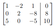A system of equations written as an augmented matrix

Row operation example (these are augmented)

$$\left[\begin{array}{cccc}1& -2& 1& 0\\ 0& 2& -8& 8\\ 5& 0& -5& 0\end{array}\right]\left[\begin{array}{cccc}1& -2& 1& 0\\ 0& 2& -8& 8\\ 0& -10& 10& 10\end{array}\right]\left[\begin{array}{cccc}1& -2& 1& 0\\ 0& 2& -8& 8\\ 0& -10& 10& 10\end{array}\right]\left[\begin{array}{cccc}1& -2& 1& 0\\ 0& 2& -8& 8\\ 0& 0& 30& -30\end{array}\right]$$ $$\left[\begin{array}{cccc}1& -2& 1& 0\\ 0& 1& -4& 4\\ 0& 0& 1& -1\end{array}\right]\left[\begin{array}{cccc}1& -2& 1& 0\\ 0& 1& 0& 0\\ 0& 0& 1& -1\end{array}\right]\left[\begin{array}{cccc}1& 0& 0& 1\\ 0& 1& 0& 0\\ 0& 0& 1& -1\end{array}\right]$$

A linear system is considered consistent if it has $>=1$ solution(s) If two matrices are row equivalent they have the same solution set, meaning that one can be transformed into the other

Row Reduction and Echelon Forms

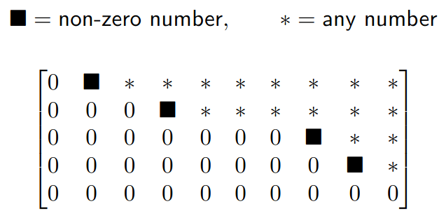
A rectangular matrix is in echelon form if

1. If there are any, all zero rows are at the bottom
2. The first non-zero entry (leading entry) of a row is to the right of any leading entries in the row above it
3. All elements below a leading entry are zero For reduced row echelon form
4. All leading entries, if any, are equal to 1.
5. Leading entries are the only nonzero entry in their respective column.

Pivots and Free Variables

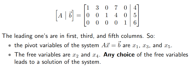
Pivot position in a matrix A is a location in A that corresponds to a leading 1 in the REF of A Pivot column is the column of the pivot

Free variables are the variables of the non-pivot columns Any choice of the free variables leads to a solution of the system ^[If you have any free variables you do not have a unique solution]

Theorem for Consistency

A linear system is consistent iff the last column of the augmented matrix does not have a pivot. This is the same as saying that the RREF of the augmented matrix does not have a row of the form $[0000...|1]$

Moreover, if a linear system is consistent, then it has 1. a unique solution iff there are no free variables. 2. infinitely many solutions that are parameterized by free variables

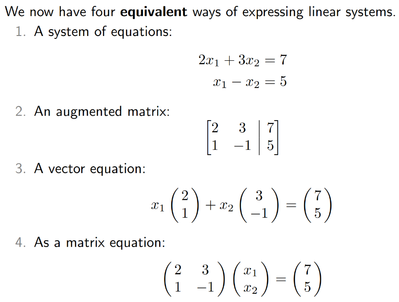
Vector Equations

$\mathbb{R}$ is all real numbers ${\mathbb{R}}^n$ is $n$ dimensions of $\mathbb{R}$ ${\mathbb{R}}^{n\times m}$ is $n$ rows and $m$ columns

Linear Combination

Linear Combination

Let $c_i\in \mathbb{R}\wedge {\vec{v}}_i\in {\mathbb{R}}^{>=1}$ $c_1{\vec{v}}_1+...c_n{\vec{v}}_n=\vec{B}$ is a linear combination of the $v$ vectors, with weights of the $c$‘s

Link to original

Span

• The set of all linear combinations of the $v$‘s in called the span of the $v$‘s
• e.g.

$$SPAN(\left[\begin{array}{c}1\\ 0\end{array}\right],\left[\begin{array}{c}0\\ 1\end{array}\right])={\mathbb{R}}^2$$

• any 2 vectors in ${\mathbb{R}}^2$ that are not scalar multiplies of each other span ${\mathbb{R}}^2$ Q: Is $\vec{b}\in SPAN({\vec{a}}_1,{\vec{a}}_2)$

$$\vec{b}=\left[\begin{array}{c}7\\ 4\\ 3\end{array}\right],{\vec{a}}_1=\left[\begin{array}{c}1\\ -2\\ -5\end{array}\right],{\vec{a}}_2=\left[\begin{array}{c}2\\ 5\\ 6\end{array}\right]$$

Matrix below in form of system of equations where X and Y scale columns 0 and 1, and column 2 are coefficients on the right hand side of the equation. By reducing this matrix to RREF, we can systematically reveal the values of X and Y

$$\left[\begin{array}{ccc}1& 2& 7\\ -2& 5& 4\\ -5& 6& 3\end{array}\right]\left[\begin{array}{ccc}1& 2& 7\\ 0& 9& 18\\ -5& 6& 3\end{array}\right]\left[\begin{array}{ccc}1& 2& 7\\ 0& 1& 2\\ -5& 6& 3\end{array}\right]\left[\begin{array}{ccc}1& 2& 7\\ 0& 1& 2\\ 0& 16& 38\end{array}\right]\left[\begin{array}{ccc}1& 2& 7\\ 0& 1& 2\\ 0& 0& 0\end{array}\right]\left[\begin{array}{ccc}1& 0& 3\\ 0& 1& 2\\ 0& 0& 0\end{array}\right]$$

Yes.

$\vec{A}\vec{x}=\vec{b}$ exists

$$\left[\begin{array}{ccc}2& 3& 7\\ 1& -1& 5\end{array}\right]\left[\begin{array}{ccc}5& 0& 22\\ 1& -1& 5\end{array}\right]\left[\begin{array}{ccc}1& 0& 22/5\\ 0& 1& 22/5-5\end{array}\right]$$

Homogeneous vs Inhomogeneous

Homogeneous: $\vec{A}\vec{x}=\vec{0}$ Homogeneous systems always have a trivial $\vec{0}$ solution, so naturally we would like to know if there are nontrivial, perhaps infinite solutions, namely if there is a free variable and a column with no pivots

Parametric vector forms of solutions to linear systems

You can parameterize the free variables and then write the solution as a vector sum.

The solution is $\vec{x}$ which is $x_1=2x_3,x_2=-x_3,x_3=x_3$ Let $x_3=t$

$$\vec{x}=\left[\begin{array}{c}2\\ -1\\ 1\end{array}\right]t$$

Nonhomogenous System

Because right side of augmented is nonzero:

$$\left[\begin{array}{cccc}1& 3& 1& 9\\ 2& -1& -5& 11\\ 0& 1& -2& 6\end{array}\right]{\to }^{RREF}\left[\begin{array}{cccc}1& 0& -2& 6\\ 0& 1& 1& 1\\ 0& 0& 0& 0\end{array}\right]$$

Let $x_3=t$

$$\vec{x}=\left[\begin{array}{c}{x}_1\\ x_2\\ x_3\end{array}\right]=\left[\begin{array}{c}2\\ -1\\ 1\end{array}\right]t+\left[\begin{array}{c}6\\ 1\\ 0\end{array}\right]$$

Linear Independence

Given $\vec{A}\vec{x}=\vec{0}$, if the only solution $\vec{x}$ is $\vec{0}$ $⟹$ Linearly Independent

Note: (This might just be wrong) \vec{A} = [\vec{a_0}\ ... \vec{a_n}]\ \big{|}\ \vec{a_i} \in \mathbb{R}^n $\wedge$ $span([\overrightarrow{a_0}...\overrightarrow{a_n}])={\mathbb{R}}^n$ ^[Same as having n rows of pivots] $⟺$ Linearly Independent

Dependence

• Any of the vectors in the set are a linear combination of the others
• If there is a free variable, so there are infinite solutions to the homogenous equation
• If the columns of A are in ${\mathbb{R}}^n$, and there are $n$ basis vectors in ${\mathbb{R}}^n$ (which is always true), then if the amount of columns in A exceeds the amount of basis vectors that exist in that dimension, it means that there are free variables, which indicates linear dependence
• If one or more of the columns of A is $\vec{0}$

Geometric interpretation of linearly independent vectors

If two vectors are linearly independent, the are not colinear If 3, then not coplanal If 4, not cospacial

Intro to Linear Transformations

Linear Transformation

$A\in R^{m\times n}$ Linear transformation $T:{\mathbb{R}}^n\to {\mathbb{R}}^m,T(\vec{v})=A\vec{v}$

• Domain of T is ${\mathbb{R}}^n$ (where we start)
• Codomain or target of T is ${\mathbb{R}}^m$
• The vector $T(\vec{x})$ is the image of $\vec{x}$ under T
• The set of all possible images is called the range
• image $\in$ range $\in$ codomain
• When the domain and codomain are both $\mathbb{R}$, you can represent them as a Cartesian Graph in ${\mathbb{R}}^2$, as in a mapping of $\mathbb{R}\to \mathbb{R}$
  • If y is the codomain and x is the domain, the range is the range, the domain is all the images of f(x)

The interpretation of matrix multiplication as a linear transformation

$$A=\left[\begin{array}{cc}1& 1\\ 0& 1\\ 1& 1\end{array}\right],\vec{u}=\left[\begin{array}{c}3\\ 4\end{array}\right],\vec{b}=\left[\begin{array}{c}7\\ 5\\ 7\end{array}\right]$$ $$T:{\mathbb{R}}^2\to {\mathbb{R}}^3$$

Compute $T(\vec{u})$

$$A\vec{u}=\left[\begin{array}{cc}1& 1\\ 0& 1\\ 1& 1\end{array}\right]\left[\begin{array}{c}3\\ 4\end{array}\right]=\left[\begin{array}{c}7\\ 4\\ 7\end{array}\right]$$

Calculate $\vec{v}\in {\mathbb{R}}^2$ so that $T(\vec{v})=\vec{b}$

$$A\vec{v}=\vec{b}$$ $$\left[\begin{array}{ccc}1& 1& 7\\ 0& 1& 5\\ 1& 1& 7\end{array}\right]\left[\begin{array}{ccc}1& 0& 2\\ 0& 1& 5\\ 1& 1& 7\end{array}\right]\left[\begin{array}{ccc}1& 0& 2\\ 0& 1& 5\\ 0& 1& 5\end{array}\right]\left[\begin{array}{ccc}1& 0& 2\\ 0& 1& 5\\ 0& 0& 0\end{array}\right]\left[\begin{array}{ccc}1& 0& 2\\ 0& 1& 5\end{array}\right]$$ $$\vec{v}=\left[\begin{array}{c}2\\ 5\end{array}\right]$$

Give a $\vec{c}\in {\mathbb{R}}^3|\neg \exists \vec{v}|T(\vec{v})=\vec{c}$ $\vee$ Give a $\vec{c}$ that is not in the range of $T$ $\vee$ Give a $\vec{c}$ that is not in the span of the columns of $A$ (Same question for all)

Range of $T$ is a bunch of images of the following form:

$$A\vec{v}=\left[\begin{array}{c}{v}_1+v_2\\ v_2\\ v_1+v_2\end{array}\right]$$

For $\vec{c}$ to not be in the range of $T$, it cannot be in the above form, e.g. it can be

$$\left[\begin{array}{c}1\\ 2\\ 3\end{array}\right]$$

Linear

A function $T:{\mathbb{R}}^n\to m$ is linear if

• T(u + v) = T(u) + T(v)
• T(c$\vec{v}$) = cT(v)
• “Principle of Superposition”
  • If we know $T(e_1)$, …, $T(e_n)$ then we know every T(v)
• Prove it is linear by proving the addition and multiplication rules

Matrix of Linear Transformations

The standard (basis) vectors

Standard vectors in ${\mathbb{R}}^n$ have a one entry for each dimension, and zeros for the rest, e.g. for ${\mathbb{R}}^3$: $\overrightarrow{e_1},\overrightarrow{e_2},\overrightarrow{e_3}=\hat{i},\hat{j},\hat{k}$

Standard matrix

Theorem

Let $T:{\mathbb{R}}^n\to {\mathbb{R}}^m$ be a linear transformation. Then there is a unique matrix $A$ such that $T(\vec{x})=A\vec{x},\vec{x}\in {\mathbb{R}}^n$ In fact, $A$ is a $m\times n$ and its $j^{th}$ column is a vector $T(\overrightarrow{e_j})$ $A=[T(\overrightarrow{e_1}),T(\overrightarrow{e_2}),...T(\overrightarrow{e_n})]$

Two and three dimensional transformations in more detail.

$$T(\overrightarrow{e_1})=\left[\begin{array}{c}5\\ -7\\ 2\end{array}\right],T(\overrightarrow{e_2})=\left[\begin{array}{c}-3\\ -8\\ 0\end{array}\right]$$ $$A=\left[\begin{array}{cc}T(\overrightarrow{e_1})& T(\overrightarrow{e_2})\end{array}\right]=\left[\begin{array}{cc}5& -3\\ -7& -8\\ 2& 0\end{array}\right]$$

Find standard matrix A for T(x) = 3$\vec{x}$ for x in ${\mathbb{R}}^2$ $A\in {\mathbb{R}}^2$

$$A=\left[\begin{array}{cc}T(\overrightarrow{e_1})& T(\overrightarrow{e_2})\end{array}\right]=\left[\begin{array}{cc}\left[\begin{array}{c}3\\ 0\end{array}\right]& \left[\begin{array}{c}0\\ 3\end{array}\right]\end{array}\right]=\left[\begin{array}{cc}3& 0\\ 0& 3\end{array}\right]$$

Linear Transformation

A Transformation is a transformation $T:{\mathbb{R}}^n\to {\mathbb{R}}^m$ satisfying

$$\begin{array}{c}T(\vec{u}+\vec{v})=T(\vec{u})+T(\vec{v})\\ T(c\vec{u})=cT(\vec{u})\end{array}$$

1-1

TLDR: 1-1 $⟺$ every column of T is a pivot column

• If there is at most one location in the codomain for every location in the domain
• 1-1 iff standard matrix has pivot in every column

Onto

TLDR: Onto $⟺$ every row of T is a pivot row A linear transformation $T:{\mathbb{R}}^n\to {\mathbb{R}}^m$ is onto if there exists a location in the codomain for every location in the domain onto iff the standard matrix has a pivot in every row The matrix A has columns which span ${\mathbb{R}}^m$. The matrix A has all pivotal rows.

1-1 and Onto

need square matrix if 1-1 then onto if Onto then 1-1

Link to original

Identity and zero matrices

0 Matrix is matrix full of zeroes Identity matrix is a square matrix full of zeroes except for the diagonal, which is all ones. Multiplying with identity matrix always yields the same matrix.

Matrix algebra (sums and products, scalar multiplies, matrix powers)

Sums: same dimensions Matrix multiplication: $r_1\ast (c_1\times r_2)\ast c_2\to r_1\times c_2$, $AB\ne BA$, $AB=AC/⟹B=C$, $AB=0/⟹A=0\vee B=0$, $AB=[A{b}_{1}A{b}_2]$

Transpose of a matrix

$$A=\left[\begin{array}{cc}a& b\\ c& d\\ e& f\end{array}\right],A^T=\left[\begin{array}{ccc}a& b& c\\ d& e& f\end{array}\right]$$

Transpose Properties

$(A^T{)}^T=A$ $(A+B{)}^T+A^T+B^T$ $(sA{)}^T=s(A^T)$ $(AB{)}^T=B^T{A}^T$

Invertibility

Definition: $A\in {\mathbb{R}}^{n\times n}$ is invertible if $\exists C\in {\mathbb{R}}^{n\times n}s.t.AC=CA=I_n$

A is invertible $⟹$ A is square A is invertible $⟺$ it is row equivalent to the identity

star Linearly dependent $⟺$ Singular

• Mnemonic: After the trial, Johnny Depp was Single Linearly independent $⟺$ Invertible
• This is just the inverse of the above

also

• $A\in {\mathbb{R}}^{n\times n}$ is invertible $⟺\forall \vec{b}\exists !\vec{x}(A\vec{x}=\vec{b})$
  • Basically means that A is 1-1 and Onto, meaning that there is exactly one domain entry for every codomain entry
    • (1-1 is at most 1, Onto is at least 1, together they make exactly 1)
• $det(A)\ne 0⟺$ invertible

Inverse Properties

$(A^{-1}{)}^{-1}=A$ $(AB{)}^{-1}=B^{-1}{A}^{-1}$ $(A^T{)}^{-1}=(A^{-1}{)}^T$ $\det A=\frac{1}{\det A^{-1}}$

$2\times 2$ Inverse Shortcut

$$A=\left[\begin{array}{cc}a& b\\ c& d\end{array}\right]$$ $${\left[\begin{array}{cc}a& b\\ c& d\end{array}\right]}^{-1}=\frac{1}{det(A)}\left[\begin{array}{cc}d& -b\\ -c& a\end{array}\right]$$

Elementary Matrix

An elementary matrix, E, is one that differs by $I_n$ by one row operation.

General way to compute inverse

Row reduce $(A|I_n)$ until you get $I_n$ for A

Therefore, if $(E^n{E}^{n-1}...E_1)A=I_n$ then $(E^n{E}^{n-1}...E_1)=A^{-1}$

Invertible Matrix Theorem - Properties

Let A be an n x n matrix. These statements are all equivalent

a) A is invertible. b) A is row equivalent to I^n. c) A has n pivotal columns. (All columns are pivotal.) d) Ax = 0 has only the trivial solution. e) The columns of A are linearly independent. f) The linear transformation x → Ax is one-to-one. g) The equation Ax = b has a solution for all b in R^n. h) The columns of A span R^n. i) The linear transformation x → Ax is onto. j) There is a n x n matrix C so that CA = I_n. (A has a left inverse.) k) There is a n x n matrix D so that AD = I_n. (A has a right inverse.) l) A^T is invertible.

Abbreviated, invertible matrix theorem (IMT)

$AB=I⟹A=B^{-1},B=A^{-1},$ B is invertible, A is invertible square A invertible $⟺$

• 0 not eigenvalue of A
• $detA\ne 0$

Singular

Noninvertible

Partitioned/Block Matrix

A partitioned matrix is a matrix that you write as a matrix of matrices When doing multiplication with a block matrix, make sure the “receiving” matrix’s entries go first, to respect the lack of commutativity in matrix multiplication. See HW 2.4 if this doesn’t make sense.

Row Column Method

Let A be m x n and B be n x p matrix. Then, the (i, j) entry of AB is row_i A · col_j B. This is the Row Column Method for matrix multiplication

Notable HW Problem

LU Factorization

Triangular Matrices

Upper Triangular: Nonzero along and above Lower Triangular: Nonzero along and below

If A is an m x n matrix that can be row reduced to echelon form without row exchanges, then A = LU . L is a lower triangular m x m matrix with 1’s on the diagonal, U is an echelon form of A.

Suppose A can be row reduced to echelon form U without interchanging rows. Then, $E_p...E_{0}A=U$ $A=LU=(E_p...E_0{)}^{-1}U$ To compute the LU decomposition:

1. Reduce A to an echelon form U by a sequence of row replacement operations, if possible.
2. Place entries in L such that the same sequence of row operations reduces L to I.

Subspaces of ${\mathbb{R}}^n$

Subset

A subset of ${\mathbb{R}}^n$, for example, is any collection of vectors that are in ${\mathbb{R}}^n$

Subspace

A subset H of ${\mathbb{R}}^n$ is a subspace if it is closed within scalar multiplication and vector addition, i.e.

• $c\in \mathbb{R};\vec{u},\vec{v}\in H$
• $c\vec{u}\in H$, $\vec{u}+\vec{v}\in H$
• $\vec{0}\in H$

Columnspace

span of columns of A same as range of A

Nullspace

span of set of $\vec{x}$ that satisfy $A\vec{x}=\vec{0}$ Null $A=\{\vec{x}|A\vec{x}=\vec{0}\}$

Basis

Linearly independent vectors that span a subspace

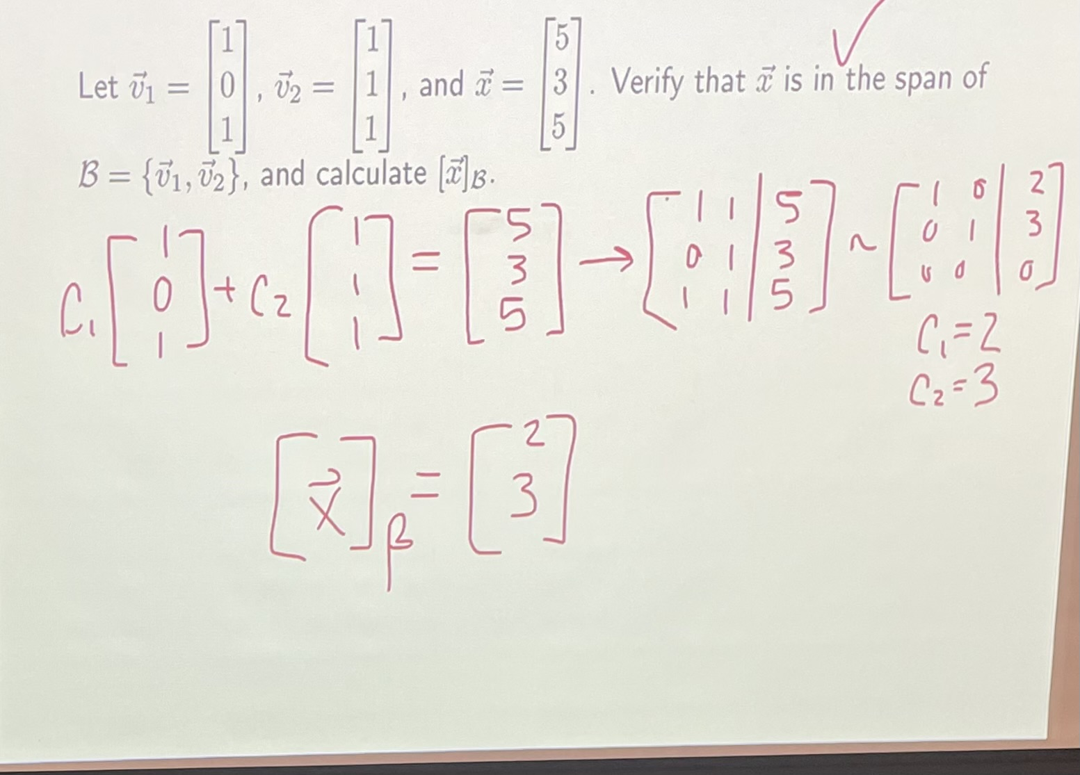
Coordinates, relative to a basis

There are many different possible choice of basis for a subspace. Our choice can give us dramatically different properties.

Standard basis are i, j, k, but you can use other vectors to span the same amount of space if you want.

1. What is a determinant? Given a linear transformation T, let us focus on the magnitude of the cross product of the basis vectors. The determinant would be the scalar factor between the original and transformed areas? (Yes)
2. If you are calculating some integral over a transformed space, is the jacobian just the determinant of the transformation, or is it related---possibly scaling the result to make sense given standard basis vectors? (Yes)

Dimension

Dimension/Cardinality of a non-zero subspace H, dim H, is the number of vectors in the basis of H. We define dim{0} = 0.

Theorem

Any two choices of ${\mathcal{B}}_1$, ${\mathcal{B}}_2$ of a non-zero subspace H have the same dimension*

Ex Problems

1. dim ${\mathbb{R}}^n$
   1. n
2. H = $\{(x_1....,x_n):x_1+...+x_n=0\}$ has dimension
   1. n - 1
   2. use the idea of # 3
   3. n variables, solve for $x_1$ ito everything else. → one pivot everything else free vars. Therefore n - 1 free vars
3. dim(Null A) is the number of
   1. number of free vars
4. dim(Col A) is the number of
   1. number of pivots

Rank

the rank of a matrix A is the dimension of its column space number of pivots

Nullity

dim(Null A) = Nullity number of of free vars

Notation from class

• Let $\mathcal{B}\in H$
  • $\mathcal{B}=\{\overrightarrow{b_1},...,\overrightarrow{b_n}\}$
  • $\mathcal{B}$ is some basis for the subspace $H$

$$\begin{array}{c}\vec{x}\in H⟹\\ \text{coords of x relative to B are c1,...,cn}\vec{x}=c_1\overrightarrow{b_1}+...+c_n\overrightarrow{b_n}\\ \\ \wedge \\ \text{coord vector of }\vec{x}\text{ relative to }\mathcal{B}[\vec{x}{]}_{\mathcal{B}}=\left[\begin{array}{c}{c}_1\\ ...\\ c_n\end{array}\right]\end{array}$$

Rank-Nullity Theorem $\star$

If a matrix A has n columns, then

$Rank(A)+Nullity(A)=n$ $dim(Col(A))+dim(Nul(A))=n$

Basis Theorem

Any two bases for a subspace have the same dimension

Invertibility Theorem

Let A be a n x n matrix. These conditions are equivalent.

1. A is invertible
2. The columns of A are a basis for ${\mathbb{R}}^n$
3. Col A = ${\mathbb{R}}^n$
4. rank A = dim Col A = n
5. Null A = {0}

Determinant

Imagine the area of parallelogram created by the basis of a standard vector space, like ${\mathbb{R}}^2$. Now apply a linear transformation $A$ to that vector space. The new area of the new parallelogram has been scaled by a factor of the determinant. $S$ is the parallelopiped.

$$area(T(S))=|det(A)|\cdot area(S)$$

You can also just think of it as the area of the parallelogram spanned by the columns of a matrix R^3 and beyond → parallelopiped and volume (assume n by n matrix because we only know how to find determinants for square matrices)

You can also get the area of S by using the determinant of the matrix created by the vectors that span S, i.e. $|\vec{a}\times \vec{b}|=area(S)⟹|det([\vec{a}\vec{b}])|=area(S)$ because you are shifting the standard basis vectors into the vector space dictated by S

Determinant Laws

• det(A) = 0 $⟺$ A is singular
  • det(A) $\ne$ 0 $⟺$ A is invertible
• det(Triangular) = product of diagonals
• det A = det $A^T$
• det(AB) = det A · det B
• $det(A^{-1})=\frac{1}{det(A)}$
• $det(kA)=k^{n}det(A)$

Determinant Post Row Operations

if A square:

• if adding rows to rows on A to get B then $detA=detB$
• if swapping rows in A to get B then $-detA=detB$
• if scaling one row of A by k, then $k\cdot det(A)$ = $det(B)$ Exactly the same for columns

Link to original

Cofactor Expansion

Cofactor expansion is a method used to calculate the Determinant of an $n\times n$ matrix $A$. It works by reducing the determinant of the $n\times n$ matrix to a sum of determinants of $(n-1)\times (n-1)$ submatrices. It is a recursive definition.

$C_{ij}=(-1{)}^{i+j}\det (M_{ij})$ where $M_{ij}$ is the determinant of the submatrix of $A$ obtained by deleting the $i$-th row and $j$-th column

The $\pm$ signs for each term of the expansion are determined solely by the position $(i,j)$ and follow a checkerboard pattern, starting with $+$ in the top-left corner

$$\left[\begin{array}{cccc}+& -& +& \cdots \\ -& +& -& \cdots \\ +& -& +& \cdots \\ ⋮& ⋮& ⋮& \ddots \end{array}\right]$$

The determinant of a matrix $A$ can be calculated by cofactor expansion along any single row $i$ or any single column $j$.

Expansion Along Row $i$: $\det (A)=a_{i1}{C}_{i1}+a_{i2}{C}_{i2}+\cdots +a_{in}{C}_{in}$

Expansion Along Column $j$: $\det (A)=a_{1j}{C}_{1j}+a_{2j}{C}_{2j}+\cdots +a_{nj}{C}_{nj}$

Strategy: To simplify calculations, it is generally best to choose the row or column with the most zeros.

Link to original

Eigenstuff

Eigenvectors and Eigenvalues

Given

1. A is square
2. $A\vec{v}$ defined, e.g. if $A\in {\mathbb{R}}^{n\times n}$ then $\vec{v}\in {\mathbb{R}}^n$

$$A\vec{v}=\lambda \vec{v}$$

Eigenvector

$\vec{v}$ is an eigenvector for $A$ An eigenvector is a vector solution $\vec{v}$ to the above equation, such that the linear transformation of $A$ has the same result as scaling the vector by $\lambda$.

Eigenvalue

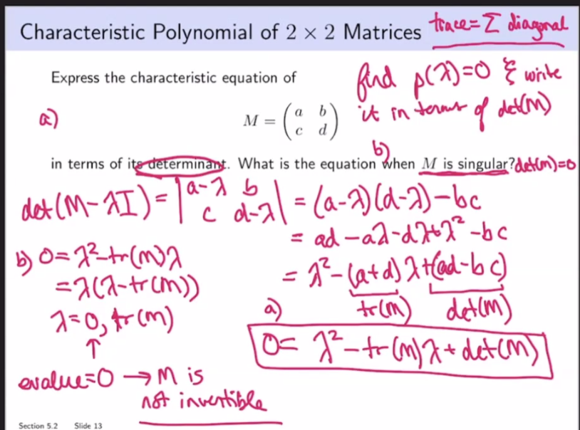
$\lambda$ is the corresponding eigenvalue ($\lambda \in \mathbb{C}$) $A\vec{v}=\lambda \vec{v}⟹\det (A-\lambda I)=0$ Solve for $\lambda$ in $\det (A-\lambda I)=0$, which yields the Characteristic Equation for this system, e.g. in a 2D systems it is ${\lambda }^2-\text{tr}A\cdot \lambda +\det A=0$. In a 3D+ system, you still have to create the characteristic equation but it requires

Notes:

• $\lambda >0⟹A\vec{v},\vec{v}$ point same direction
• $\lambda <0⟹A\vec{v},\vec{v}$ point opposite direction
• $\lambda$ can be complex even if nothing else in the equation is
• Eigenvalues cannot be determined from the reduced version of a matrix ⭐
  • i.e. row reductions change the eigenvalues of a matrix
• The diagonal elements of a triangular matrix are its eigenvalues.
• A invertible iff 0 is not an eigenvalue of A.
• Stochastic matrices have an eigenvalue equal to 1.
• If ${\vec{v}}_1,{\vec{v}}_2,...,{\vec{v}}_k$ are eigenvectors that correspond to distinct eigenvalues, then ${\vec{v}}_1,{\vec{v}}_2,...,{\vec{v}}_k$ are linearly independent

Defective

An eigenvalue is defective if and only if it does not have a complete Set of Linearly Independent eigenvectors.
$\lambda =0⟹\text{ Defective}$ Due to $\mathrm{Im}\lambda$‘s contribution, $\mathrm{Re}\lambda =0/⟹\text{ Defective}$

Neutral Eigenvalue

$$\forall \lambda s.t.\mathrm{Re}\lambda =0$$

Eigenspace

• the span of the eigenvectors that correspond to a particular eigenvalue

• $Nul(A-\lambda I)$

Link to original

Characteristic Equation

$det(A-\lambda I)=0$ to get values for $\lambda$. Recall $det(T)=0$ means noninvertible. If a matrix isn’t invertible, then we won’t get trivial solutions when solving. Also the idea of reducing the dimension through the transformation is relevant; squishing the basis vectors all onto the same span where the area/volume is 0. Recall eigenvectors remain on the same span despite a linear transformation.

$\lambda$ is an eigenvalue of A $⟺$ $(A-\lambda I)$ is singular

trace of a Matrix $tr(M)$ is the sum of diagonal

Characteristic Polynomial

$det(A-\lambda I)$ n degree polynomial → n roots → maximum n eigenvalues (could be repeated)

Algebraic Multiplicity

Algebraic multiplicity of an eigenvalue is how many times an eigenvalue repeatedly occurs as the root of the characteristic polynomial.

Geometric Multiplicity

• Geometric multiplicity of an eigenvalue is the number of eigenvectors associated with an eigenvalue; $dim(Nul(A-\lambda I))$, which is saying how many eigenvector solutions does this eigenvalue have (recall $dim(B)$ is number of free vars in $B$)

Link to original

Similar

1. square matrices A,B are similar $⟺$ we can find P so that $A=PB{P}^{-1}$
2. A,B similar $⟹$ same Characteristic Polynomial $⟹$ same eigenvalues

Link to original

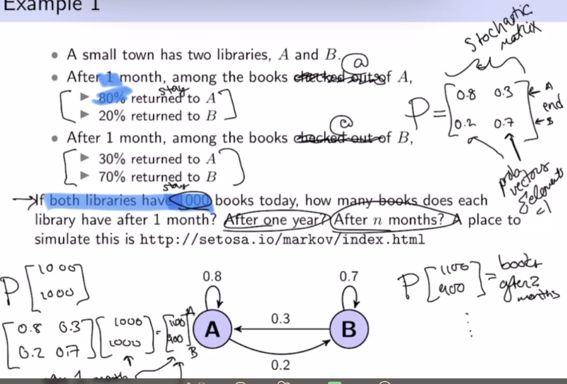
Markov chains

Stochastic matrix

• Matrix that uses the rates/probabilities
• Columns are probability vectors.
• Sum to 1

Probability Vector

Some vector $\vec{x}$ with nonnegative elements that sum to 1

Stochastic Matrix

A stochastic matrix is a square matrix, P , whose columns are probability vectors. |det(P)| ⇐ 1, only volume contracting or preserving

Markov Chain

A Markov chain is a sequence of probability vectors, and a stochastic matrix P , such that:

$$\begin{array}{c}{P}^k\overrightarrow{x_0}={\vec{x}}_k\\ {\vec{x}}_{k+1}=P{\vec{x}}_k;k=0,1,2,...\end{array}$$

Convergence

Regularity

• Stochastic matrix is regular if there $\exists (k\ge 1)P^k$ strictly has positive entries
• Regular $⟺$ unique steady state vectors
  • Irregular $⟺$ $0\le n\ne 1$ steady state vectors

Steady-State Vector

A steady-state vector for P is a vector $\vec{q}$ such that $P\vec{q}=\vec{q}$. $(P-I)\vec{q}=0$ Fixed point, I/O the same

Ex: Determine the steady state vector for

$$P=\left[\begin{array}{cc}.8& .3\\ .2& .7\end{array}\right]$$

Goal: solve $P\vec{q}=\vec{q}$ $(P-I)\vec{q}=\vec{q}$

$$\begin{array}{c}\left[\begin{array}{ccc}.8-1& .3& 0\\ .2& .7-1& 0\end{array}\right]\\ \left[\begin{array}{ccc}-.2& .3& 0\\ .2& -.3& 0\end{array}\right]\\ \left[\begin{array}{ccc}1& -\frac{3}{2}& 0\\ 0& 0& 0\end{array}\right]\end{array}$$ $$\therefore \vec{q}=t\left[\begin{array}{c}\frac{3}{2}\\ 1\end{array}\right]$$ $$\frac{3}{2}t+t=1$$ $$\therefore t=\left[\begin{array}{c}\frac{3}{5}\\ \frac{2}{5}\end{array}\right]$$

Related to eigenvectors. $\vec{q}$ is defined as $li{m}_{k\to \infty }\left(P^k\overrightarrow{x_0}\right)=\vec{q}$, also $P\vec{q}=\vec{q}$ When you reapply a linear transformation approaching infinity times, all the points in the subspace will approach the span of

1. If the transformation is regular, a single eigenvector
   1. For our regular stochastic matrices, this is what the steady state vector is.
2. If the transformation is irregular, possibly multiple eigenvectors or none at all. If multiple, points will converge to the closest possible eigenspace.

Theorem

as k → $\infty$

$${\vec{x}}_{k+1}=P{\vec{x}}_k;k=0,1,2,...$$

If $P$ is a regular stochastic matrix, then $P$ has a unique steady-state vector $\vec{q}$, and $\overrightarrow{x_{k+1}}=P\overrightarrow{x_k}$ converges to $\vec{q}$ as $k\to \infty$; $(P^k\overrightarrow{x_0}{⟶}_{k\to \infty }\vec{q})$ where $P\vec{q}=\vec{q}$

M3

Diagonalization

Diagonalizable

Complex Eigenvalues

Complex numbers

Conjugate $\overline{a+bi}=a-bi$

• Reflects across the $Re(z)$ axis Magnitude (or “Modulus”) $|a+bi|=\sqrt{a^2+b^2}=\sqrt{(a+bi)(a-bi)}$ Polar $a+ib=r(cos\varphi +isin\varphi )$ where $r$ is the magnitude

if x and y $\in \mathbb{C}$, $\vec{v}\in {\mathbb{C}}^n$

• $\overline{(x+y)}=\overline{x}+\overline{y}$
• $\overline{A\vec{v}}=A\overline{\vec{v}}$
• $Im(x\overline{x})=0$
• $\overline{(xy)}=\overline{x}\overline{y}$

Euler’s Formula

$z=|z|e^{i\varphi }$

Suppose $z_1$ has an angle ${\varphi }_1$ and $z_2$ has ${\varphi }_2$ The product $z_1{z}_2$ has angle ${\varphi }_1+{\varphi }_2$, and modulus $|z_1||z_2|$ Can use Euler’s formula to make it easier $z_1{z}_2=(|z_1|e^{i{\varphi }_1})(|z_2|e^{i{\varphi }_2})=(|z_1||z_2|e^{i({\varphi }_1+{\varphi }_2)})$

Complex Eigenvalues

Theorem: Fundamental Theorem of Algebra An $n$ degree polynomial has exactly $n$ complex roots (including multiplicity).

Theorem

• If $\lambda \in \mathbb{C}$ is a root of a real polynomial, $\overline{\lambda }$ is also
  • Complex roots come in complex conjugate pairs
• If $\lambda$ is an eigenvalue of real matrix $A$, with eigenvector $\vec{v}$, then $\overline{\lambda }$ is an eigenvalue of A with eigenvector $\overline{\vec{v}}$

Example

4 of the eigenvalues of a 7 x 7 matrix are -2, 4 + i, -4 - i, and i

• Because there are 3 nonconjugate complex pairs, we know that the remaining eigenvalues are the conjugates of the given complex values
• What is the characteristic polynomial?
• $p(\lambda )=(\lambda +2)(\lambda -(4+i))(\lambda -(-4-i))(\lambda -i)(\lambda -(4-i))(\lambda -(-4+i))(\lambda +i)$

Example

The matrix that rotates vectors by $\frac{\pi }{4}$ radians about the origin and then scales vectors by $\sqrt{2}$ is:

$$\left[\begin{array}{cc}1& -1\\ 1& 1\end{array}\right]$$

What are the eigenvalues of $A$? Find an eigenvector for each eigenvalue

$det(A-\lambda I)=(1-\lambda {)}^2={\lambda }^2-2\lambda +2$ $\lambda =\frac{2\pm \sqrt{4-8}}{2}=\frac{2\pm 2i}{2}=1\pm i$ ${\lambda }^{+}$:

$$\begin{array}{c}A-{\lambda }^{+}I\\ \left[\begin{array}{cc}1-(1+i)& -1\\ 1& 1-(1+i)\end{array}\right]\\ \left[\begin{array}{cc}-i& -1\\ 1& -i\end{array}\right]\\ \left[\begin{array}{cc}1& -i\\ -i& -1\end{array}\right]\\ \left[\begin{array}{cc}1& -i\\ 0& 0\end{array}\right]\to \overrightarrow{v_{+}}=\left[\begin{array}{c}i\\ 1\end{array}\right]\end{array}$$

${\lambda }^{-}$:

$$\begin{array}{c}""""""\to \overrightarrow{v_{-}}=\left[\begin{array}{c}-i\\ 1\end{array}\right]\end{array}$$

Could reason the eigenvalue for ${\lambda }^{-}$ by the fact that eigenvalues and their eigenvectors come in complex conjugate pairs.

Inner Product, Length, Orthogonality

Dot Product

Length

$||\vec{u}||=\sqrt{\vec{u}\cdot \vec{u}}=\sqrt{u_1^2+\cdots +u_n^2}$

Orthogonality

• $||\vec{u}+\vec{w}|{|}^2=||\vec{u}|{|}^2+||\vec{w}|{|}^2\vee \vec{u}\cdot \vec{w}=0⟹\text{Orthogonal}$
• If $W$ is a subspace of ${\mathbb{R}}^n$ and $\vec{z}\in {\mathbb{R}}^n$, $\vec{z}$ is orthogonal to $W$ if it is orthogonal to every vector in $W$
• The set of all vectors orthogonal to a subspace is a itself a subspace, called the Orthogonal Complement of $W$, $W^{\perp }$, W perp
  • $W^{\perp }=\{\vec{z}\in {\mathbb{R}}^n\mid \forall (\vec{w}\in W)\vec{z}\cdot \vec{w}=0\}$
• $dim(RowA)=dim(ColA)$
• $(RowA{)}^{\perp }=NulA$
• $(ColA{)}^{\perp }=Nul(A^T)$

$\vec{x}\in Nul(A)⟺$

• $A\vec{x}=\vec{0}$
• $\vec{x}$ is orthogonal to each row of $A$
• $RowA$ is orthogonal complement to $NulA$
• $dim(RowA)+dim(NulA)=$ number of columns

$\vec{a}\cdot \vec{b}=0\wedge \vec{a}\ne \vec{0},\vec{b}\ne 0⟺\vec{a}\perp \vec{b}⟺a\text{ and }b\text{ are Orthogonal}$

Orthogonal Sets

Orthogonal Vector Sets

A set of vectors are an orthogonal set of vectors if every pair in the set is orthogonal to every other vector in the set.

Linear Independence for Orthogonal Sets: If there is an orthogonal set of vectors $O$, then

$$||c_1\cdot {\vec{u}}_1+\cdots +c_n\cdot {\vec{u}}_n|{|}^2=c_1^2\cdot ||{\vec{u}}_1|{|}^2+\cdots +c_n^2\cdot ||{\vec{u}}_n|{|}^2$$

$\vec{0}\notin O⟹O$ lin. indep.

Expansion in Orthogonal Basis If $O$ is the basis for subspace $W$ in ${\mathbb{R}}^n$ and $O$ is an orthogonal basis, then for any vector $\vec{w}\in W$

$$\vec{w}=c_1{\vec{u}}_1+\cdots +c_n{\vec{u}}_n$$ $$c_i=\frac{\vec{w}\cdot {\vec{u}}_i}{{\vec{u}}_i\cdot {\vec{u}}_i}$$

Orthogonal Projection

Orthogonal Decomposition

Best Approximation

Gram-Schmidt Process

QR Factorization

Least Squares

Exam 4

Google Page Rank

Symmetric Matrix

Spectral Decomposition

Orthogonal Diagonalization

Quadratic Form

Constrained Optimization

Singular Value Decomposition