Systems of Differential Equations

2D Homogeneous Linear Systems with Constant Coefficients

$$\frac{d\vec{x}}{dt}=A\vec{x}\text{where }\vec{x}(t)=\left[\begin{array}{c}{x}_1(t)\\ x_2(t)\end{array}\right],A\text{ is a }2\times 2\text{ real constant matrix}$$

Distinct Real & Nonzero Eigenvalues

Loosey goosey explanation

Recall $u^{\prime }=\lambda u⟹u=c{e}^{\lambda t}$ “Think of matrices as a generalization of the number system” Well it turns out that ${\vec{x}}^{\prime }=A\vec{x}⟹\vec{x}=\vec{c}{e}^{At}$, where $\dim A=2$ A is diagonalizable $⟺\vec{x}=c_1{e}^{{\lambda }_{1}t}{\vec{x}}_1+c_2{e}^{{\lambda }_{2}t}{\vec{x}}_2$ where ${\lambda }_n$ are A’s eigenvalues, and ${\vec{v}}_n$ are $A$‘s eigenvectors. See Eigenvectors, Eigenvalues, and Eigenspaces.

Find the eigenvalues of $A$ by solving the Characteristic Polynomial We assume that $\lambda ={\lambda }_1,{\lambda }_2\in \mathbb{R}\ne 0{\lambda }_1\ne {\lambda }_2$

$$\begin{array}{r}\det (A-\lambda I)=0\end{array}$$

We find ${\lambda }_1$‘s eigenvector ${\vec{u}}_1$ by solving $(A-{\lambda }_{1}I)\vec{x}=0$ We find ${\lambda }_2$‘s eigenvector ${\vec{u}}_1$ by solving $(A-{\lambda }_{2}I)\vec{x}=0$ The general solution for $\vec{x}$ is

$$\vec{x}(t)=C_1\exp ({\lambda }_{1}t){\vec{u}}_1+C_2\exp ({\lambda }_{2}t){\vec{u}}_2\text{where }{C}_1,C_2\text{ are free parameters}$$

If an initial condition is given, then there is a unique solution.

Stability & Phase Portrait

Col

![[Pasted image 20250905173724.png|${\lambda }_1,{\lambda }_2<0⟹$Stable Nodal Sink, Asymptotically Stable]]

![[Pasted image 20250905173930.png|${\lambda }_1,{\lambda }_2>0⟹$ Nodal Source, Unstable]]

![[Pasted image 20250905180026.png|${\lambda }_1>0{\lambda }_2<0⟹$ Saddle, Unstable]]

A Zero Eigenvalue

This is a specific case of the previous section. This is the same as the previous section Distinct Real & Nonzero Eigenvalues, except We assume $\lambda ={\lambda }_1,{\lambda }_2,\text{WLOG }{\lambda }_1=0,{\lambda }_2\ne {\lambda }_1$, which implies

$$\vec{x}=C_1{\vec{u}}_1+C_2\exp ({\lambda }_{2}t){\vec{u}}_2$$

This is a simplification of the general formula from Distinct Real & Nonzero Eigenvalues On the eigenspace of the zero eigenvalue ${\lambda }_1$, the solutions are time independent; i.e., the eigenspace of the zero eigenvalue is a line of equilibrium. The other eigenvalue determines the behavior of the phase space outside of the equilibrium line.

Stability & Phase Portrait

Both cases have ${\lambda }_1=0$

Col

![[Pasted image 20250912160920.png|${\lambda }_2<0$, Attractive line of equilibirum, strictly stable|225]]

![[Pasted image 20250912160948.png|${\lambda }_2>0$, Repulsive line of equilibrium, unstable|200]]

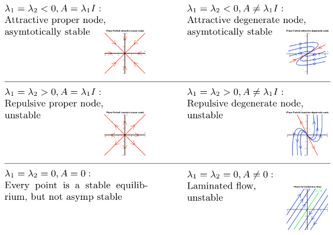
Repeated Real Eigenvalues

This is the same as the previous sections except We assume $\lambda ={\lambda }_1,{\lambda }_2\in \mathbb{R},{\lambda }_1={\lambda }_2$

Easy Case

where $A={\lambda }_{1}I$

$$\vec{x}=\exp ({\lambda }_{1}t)\vec{C}$$

This is a simplification of the general formula from Distinct Real & Nonzero Eigenvalues, where $\vec{C}$ is formed by $C_1$ and $C_2$, and we chose the Standard Basis Vectors for our eigenvectors, because any linearly independent pair of vectors in ${\mathbb{R}}^2$ would be satisfactory.

Hard Case

where $A\ne {\lambda }_{1}I$

$$\vec{x}=C_1\exp ({\lambda }_{1}t)\vec{u}+C_2\exp ({\lambda }_{1}t)\left(\vec{v}+t\vec{u}\right)$$

We get the first term for this general solution from the typical method of finding eigenvectors, but because we have multiplicity of 2, our result is only one eigenspace, i.e. a partial solution. In order to get a full solution, we have to find a generalized eigenvector as well (the eigenvector for the second term). We get this eigenvector $\vec{v}$ by solving $(A-{\lambda }_{1}I)\vec{x}=\vec{u}$, where $\vec{u}$ was the eigenvector from the first term.

Stability and Phase Portrait

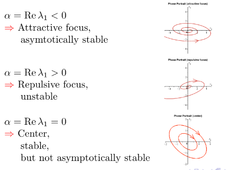
Complex Eigenvalues

This is the same as the previous sections except We assume $\lambda ={\lambda }_1,{\lambda }_2\in \mathbb{C},{\lambda }_1=\alpha +\beta i,{\lambda }_2=\alpha -\beta i,\beta \ne 0$

$$\text{Complex-valued: }\vec{x}=C_1\exp ({\lambda }_{1}t){\vec{u}}_1+C_2\exp ({\lambda }_{2}t){\vec{u}}_2$$ $$\text{Real-valued: }\vec{x}=C_1\mathrm{Re}(\exp ({\lambda }_{1}t){\vec{u}}_1)+C_2\mathrm{Im}(\exp ({\lambda }_{1}t){\vec{u}}_1)=C_1\exp (\alpha t)\left(\cos (\beta t)\vec{a}-\sin (\beta t)\vec{b}\right)+C_2\exp (\alpha t)\left(\sin (\beta t)\vec{a}+\cos (\beta t)\vec{b}\right)$$

where $\exp ({\lambda }_{1}t){\vec{u}}_1$ is a complex solution to the system where $\alpha =\mathrm{Re}{\lambda }_1$ gives the growth/decay rate where $\beta =\mathrm{Im}{\lambda }_1$ is the frequency of the oscillation of the system

When finding eigenvectors, for $A\in {\mathbb{C}}^{2\times 2}$ and $\det A\ne 0$, ignore the second row, because it can be eliminated by definition. See Misc. When you get $\lambda =\alpha \pm \beta i$, you can use either eigenvalue-eigenvector pair for the general equation. They will both give you the same solution, as the sign change will get absorbed in the $C$s

Stability and Phase Portrait

Apply matrix $A$ once, to get the initial velocity, to determine the direction of rotation $\exp \alpha t$ scales the whole solution

Link to original

Shifted Systems of Linear Differential Equations

$${\vec{x}}^{\prime }=A(\vec{x}-\vec{a})\text{and}{\vec{x}}^{\prime }=A\vec{x}+\vec{b}$$

Transient Method

Substitute a variable into the system, so that we have a problem we know how to solve. Similar idea to U Substitution. Solution: Equilibrium + Transient

Type 1

${\vec{x}}^{\prime }=A(\vec{x}-\vec{a})$, where A is a constant square matrix, $\vec{a}$ is a constant vector Set $\vec{y}=\vec{x}-\vec{a}$, as $\vec{a}$ is an equilibrium, and $\vec{y}$ is the transient solution Solve for $\vec{y}(t)$ from ${\vec{y}}^{\prime }=A\vec{y}$. See 2D Homogeneous Linear Systems with Constant Coefficients Solution is $\vec{x}(t)=\vec{a}+\vec{y}(t)$

Example

$$\left[\begin{array}{c}{x}_1^{\prime }\\ x_2^{\prime }\end{array}\right]=\left[\begin{array}{cc}3& -3\\ -1& 5\end{array}\right]\left[\begin{array}{c}{x}_1-2\\ x_2-3\end{array}\right]$$

(a) Find all equilibria (b) Find general solutions (c) Solve with the initial condition $\vec{x}=\left[\begin{array}{c}1\\ 0\end{array}\right]$ (d) Sketch the phase portrait (e) Determine the stability of each equilibrium

(a) This ODE is of the form ${\vec{x}}^{\prime }=A(\vec{x}-\vec{a})$, i.e. Type 1, so the equilbrium is $\vec{a}=\left[\begin{array}{c}2\\ 3\end{array}\right]⟹(2,3)$ (b) Let $\vec{y}=\vec{x}-\vec{a}$, so we have ${\vec{y}}^{\prime }=A\vec{y}$, which we know how to solve because it is a 2D Homogeneous Linear Systems with Constant Coefficients. Eigenvalues = $\det (A-\lambda I)=0⟹\lambda =2,6$ Eigenvectors = $(A-{\lambda }_{i}I){\vec{u}}_i=\vec{0}⟹\vec{u}=\left[\begin{array}{c}3\\ 1\end{array}\right],\left[\begin{array}{c}-1\\ 1\end{array}\right]$

$$\therefore \vec{y}(t)=C_1\exp (2t)\left[\begin{array}{c}3\\ 1\end{array}\right]+C_2\exp (6t)\left[\begin{array}{c}-1\\ 1\end{array}\right]$$ $$⟹\boxed{\vec{x}(t)=\left[\begin{array}{c}2\\ 3\end{array}\right]+C_1\exp (2t)\left[\begin{array}{c}3\\ 1\end{array}\right]+C_2\exp (6t)\left[\begin{array}{c}-1\\ 1\end{array}\right]}$$

(c)

$$\vec{x}(0)=\left[\begin{array}{c}1\\ 0\end{array}\right]=\left[\begin{array}{c}2\\ 3\end{array}\right]+C_1\exp (2(0))\left[\begin{array}{c}3\\ 1\end{array}\right]+C_2\exp (6(0))\left[\begin{array}{c}-1\\ 1\end{array}\right]$$ $$\left[\begin{array}{c}1\\ 0\end{array}\right]=\left[\begin{array}{c}2\\ 3\end{array}\right]+C_1\left[\begin{array}{c}3\\ 1\end{array}\right]+C_2\left[\begin{array}{c}-1\\ 1\end{array}\right]⟹C_1=-1,C_2=-2$$ $$\vec{x}(t)=\left[\begin{array}{c}2\\ 3\end{array}\right]-\exp (2t)\left[\begin{array}{c}3\\ 1\end{array}\right]-2\exp (6t)\left[\begin{array}{c}-1\\ 1\end{array}\right]$$

(d) Center the portrait at the equilibrium point $(2,3)$ Both eigenvalues are postitive, so the eigenspace arrows all go out. Because they have the same sign, the curves off of the eigenspaces are parabolas. (e) The equilibrium is unstable.

Type 2

${\vec{x}}^{\prime }=A\vec{x}+\vec{b}$, where A is a constant square matrix, $\vec{b}$ is a constant vector Essentially, convert into Type 1 by finding an equilibrium $\vec{a}$ by solving $A\vec{x}+\vec{b}=\vec{0}$ for $\vec{x}$. If no equilbrium exists, you must use Variation of Parameters instead. Transient solution $\vec{y}=\vec{x}-\vec{a}$ that satisfies ${\vec{y}}^{\prime }=A\vec{y}$, solve for $\vec{y}(t)$. See 2D Homogeneous Linear Systems with Constant Coefficients Solution is $\vec{x}(t)=\vec{a}+\vec{y}(t)$

Link to original

2D Nonlinear Systems of Differential Equations

$$\left[\begin{array}{c}{x}^{\prime }\\ y^{\prime }\end{array}\right]=\vec{F}(x,y)=\left[\begin{array}{c}f(x,y)\\ g(x,y)\end{array}\right]$$

Equilibria

Find the equilibria by solving for all $(x,y)$ that satisfy $\vec{F}=\vec{0}$

Linearization

Find the Linearization of the system.

$$\left[\begin{array}{c}{x}^{\prime }\\ y^{\prime }\end{array}\right]=\left[\begin{array}{c}f(x,y)\\ g(x,y)\end{array}\right]⟹\left[\begin{array}{c}{x}^{\prime }\\ y^{\prime }\end{array}\right]=\vec{F}(\text{EP})+J_{\vec{F}(\text{EP})}\left[\begin{array}{c}x-\text{EP.x}\\ y-\text{EP.y}\end{array}\right]$$

where $J_{\vec{F}(EP)}$ is the Jacobian matrix at a particular equilibrium point

where EP is each Equilibrium Point, where EP.x and EP.y are the x and y components

By definition at an equilibrium point, the function is equal to $\vec{0}$. See Equilibria.

Therefore the linearization becomes this:

$$\left[\begin{array}{c}{x}^{\prime }\\ y^{\prime }\end{array}\right]=J_{\vec{F}(\text{EP})}\left[\begin{array}{c}x-\text{EP.x}\\ y-\text{EP.y}\end{array}\right]$$ $$J_{\vec{F}(\text{EP})}=\left[\begin{array}{cc}{f}_x& f_y\\ g_x& g_y\end{array}\right]@\text{EP}$$

The final expression for the linearization looks like this.

$$\left[\begin{array}{c}{x}^{\prime }\\ y^{\prime }\end{array}\right]=\left(\left[\begin{array}{cc}{f}_x& f_y\\ g_x& g_y\end{array}\right]@\text{EP}\right)\left[\begin{array}{c}x-\text{EP.x}\\ y-\text{EP.y}\end{array}\right]$$

This is a Shifted Systems of Linear Differential Equations

Perterbation

Given

$${\vec{v}}^{\prime }=A\vec{v}$$

Which is the exact form of the homogenous part of our Linearization, except we have

$$\vec{v}=J_{\vec{F}(\text{EP})}(\vec{v}-\text{EP})$$

Neutral Eigenvalues ($\mathrm{Re}\lambda =0$) lead to structural instability, e.g. a perterbation leads to signficant change.

Approximating Dynamics

Given

$$\vec{v}=J_{\vec{F}(\text{EP})}(\vec{v}-\text{EP})$$

We approximate the dynamics of the original system, by finding the dynamics of the Linearization TLDR: We find the Eigenstuff of the Jacobian, and use that to construct our Phase Portrait

Lotka-Volterra Competition Model

$$\frac{d🐺}{dt}=g_{🐺}🐺\left(1-\frac{🐺}{K_{🐺}}-{\alpha }_{🐺🐯}\frac{🐯}{K_{🐺}}\right)$$ $$\frac{d🐯}{dt}=r_{🐯}🐯\left(1-\frac{🐯}{K_{🐯}}-{\alpha }_{🐯🐺}\frac{🐺}{K_{🐯}}\right)$$

where $🐺$, $🐯$ are population sizes

where $g_{🐺}$, $r_{🐯}$ are intrinsic per capita growth rates

where $K_{🐺}$, $K_{🐯}$ are carrying capacities.

where ${\alpha }_{🐺🐯}$, ${\alpha }_{🐯🐺}$ are competition coefficients

• where ${\alpha }_{🐺🐯}$ measures the negative effect tigers have on wolves
• where ${\alpha }_{🐯🐺}$ measures the native effect wolves have on tigers

Lotka-Volterra Predator-Prey Model

$$\frac{d🐰}{dt}=\alpha 🐰-\beta 🐰🐺$$ $$\frac{d🐺}{dt}=\delta 🐰🐺-\gamma 🐺$$

where🐰 is the prey population size

where 🐺 is the predator population size

where $\alpha$ is the prey growth rate (birth rate)

where $\beta$ is the predation rate/interaction rate

where $\gamma$ is the predator death rate

where $\delta$ is the conversion efficiency of prey into new predators.

Link to original

Misc

• $(\det A\ne 0⟺\text{lin. indep.})⟹\text{Equilibrium only @ }\vec{0}$
• Decaying eigenvector scalars decay the eigenspace, growing ones grow the whole eigenspace.